Douglas C. Montgomery - Introduction to Linear Regression Analysis

Other abuses of regression are discussed in subsequent chapters. For further reading on this subject, see the article by Box [1966].

Some regression situations seem to imply that a straight line passing through the origin should be fit to the data. A no-intercept regression modeloften seems appropriate in analyzing data from chemical and other manufacturing processes. For example, the yield of a chemical process is zero when the process operating temperature is zero.

The no-intercept model is

(2.48)

Given n observations ( yi , xi ), i = 1, 2, …, n , the least-squares function is

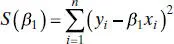
The only normal equation is

(2.49)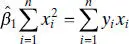

and the least-squares estimator of the slopeis

(2.50)

The estimator of is unbiased for β 1, and the fitted regression modelis

(2.51)

The estimator of σ 2is

(2.52)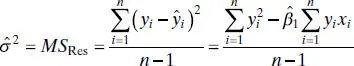

with n − 1 degrees of freedom.

Making the normality assumption on the errors, we may test hypotheses and construct confidence and prediction intervals for the no-intercept model. The 100(1 − α) percent CI on β 1is

(2.53)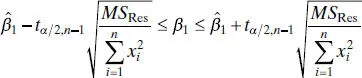

A 100(1 − α) percent CI on E(y|x0), the mean response at x = x 0, is

(2.54)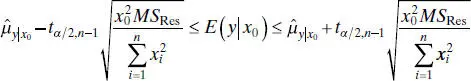

The 100(1 − α) percent prediction interval on a future observation at x = x0, say y 0, is

(2.55)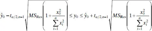

Both the CI (2.54)and the prediction interval (2.55)widen as x 0increases. Furthermore, the length of the CI (2.54)at x = 0 is zero because the model assumes that the mean y at x = 0 is known with certainty to be zero. This behavior is considerably different than observed in the intercept model. The prediction interval (2.55)has nonzero length at x 0= 0 because the random error in the future observation must be taken into account.

It is relatively easy to misuse the no-intercept model, particularly in situations where the data lie in a region of x space remote from the origin. For example, consider the no-intercept fit in the scatter diagram of chemical process yield ( y ) and operating temperature ( x ) in Figure 2.12 a . Although over the range of the regressor variable 100°F ≤ x ≤ 200°F, yield and temperature seem to be linearly related, forcing the model to go through the origin provides a visibly poor fit. A model containing an intercept, such as illustrated in Figure 2.12 b , provides a much better fit in the region of x space where the data were collected.

Frequently the relationship between y and x is quite different near the origin than it is in the region of x space containing the data. This is illustrated in Figure 2.13for the chemical process data. Here it would seem that either a quadratic or a more complex nonlinear regression model would be required to adequately express the relationship between y and x over the entire range of x . Such a model should only be entertained if the range of x in the data is sufficiently close to the origin.

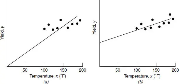
Figure 2.12 Scatter diagrams and regression lines for chemical process yield and operating temperature: ( a ) no-intercept model; ( b ) intercept model.

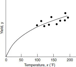
Figure 2.13 True relationship between yield and temperature.

The scatter diagram sometimes provides guidance in deciding whether or not to fit the no-intercept model. Alternatively we may fit both models and choose between them based on the quality of the fit. If the hypothesis β 0= 0 cannot be rejected in the intercept model, this is an indication that the fit may be improved by using the no-intercept model. The residual mean square is a useful way to compare the quality of fit. The model having the smaller residual mean square is the best fit in the sense that it minimizes the estimate of the variance of y about the regression line.

Generally R 2is not a good comparative statistic for the two models. For the intercept model we have

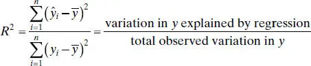
Note that R 2indicates the proportion of variability around explained by regression. In the no-intercept case the fundamental analysis-of-variance identity (2.32)becomes

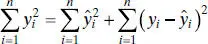
so that the no-intercept model analogue for R 2would be

The statistic indicates the proportion of variability around the origin(zero) accounted for by regression. We occasionally find that is larger than R 2even though the residual mean square (which is a reasonable measure of the overall quality of the fit) for the intercept model is smaller than the residual mean square for the no-intercept model. This arises because is computed using uncorrected sums of squares.