Douglas C. Montgomery - Introduction to Linear Regression Analysis

That is, the conditional distribution of y given x is normal with conditional mean

(2.63)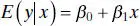

and conditional variance . Note that the mean of the conditional distribution of y given x is a straight-line regression model. Furthermore, there is a relationship between the correlation coefficient ρ and the slope β 1. From Eq. (2.62b) we see that if ρ = 0, then β 1= 0, which implies that there is no linear regression of y on x . That is, knowledge of x does not assist us in predicting y .

The method of maximum likelihood may be used to estimate the parameters β 0and β 1. It may be shown that the maximum-likelihood estimators of these parameters are

(2.64a)

and

(2.64b)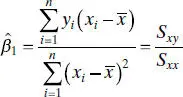

The estimators of the intercept and slope in Eq. (2.64)are identical to those given by the method of least squares in the case where x was assumed to be a controllable variable. In general, the regression model with y and x jointly normally distributed may be analyzed by the methods presented previously for the model where x is a controllable variable. This follows because the random variable y given x is independently and normally distributed with mean β 0+ β 1 x and constant variance . As noted in Section 2.12.1, these results will also hold for anyjoint distribution of y and x such that the conditional distribution of y given x is normal.

It is possible to draw inferences about the correlation coefficient ρ in this model. The estimator of ρ is the sample correlation coefficient

(2.65)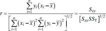

Note that

(2.66)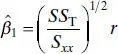

so that the slope is just the sample correlation coefficient r multiplied by a scale factor that is the square root of the spread of the y ’s divided by the spread of the x ’s. Thus, and r are closely related, although they provide somewhat different information. The sample correlation coefficient r is a measure of the linear associationbetween y and x, while measures the change in the mean of y for a unit change in x . In the case of a controllable variable x, r has no meaning because the magnitude of r depends on the choice of spacing for x . We may also write, from Eq. (2.66),

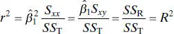
which we recognize from Eq. (2.47)as the coefficient of determination. That is, the coefficient of determination R 2is just the square of the correlation coefficient between y and x .

While regression and correlation are closely related, regression is a more powerful tool in many situations. Correlation is only a measure of association and is of little use in prediction. However, regression methods are useful in developing quantitative relationships between variables, which can be used in prediction.

It is often useful to test the hypothesis that the correlation coefficient equals zero, that is,

(2.67)

The appropriate test statistic for this hypothesis is

(2.68)

which follows the t distribution with n − 2 degrees of freedom if H 0: ρ = 0 is true. Therefore, we would reject the null hypothesis if | t 0| > t α/2, n−2. This test is equivalent to the t test for H 0: β 1= 0 given in Section 2.3. This equivalence follows directly from Eq. (2.66).

The test procedure for the hypotheses

(2.69)

where ρ 0≠ 0 is somewhat more complicated. For moderately large samples (e.g., n ≥ 25) the statistic

(2.70)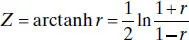

is approximately normally distributed with mean

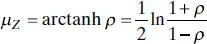
and variance

Therefore, to test the hypothesis H 0: ρ = ρ 0, we may compute the statistic

(2.71)

and reject H 0: ρ = ρ 0if | Z 0| > Z α/2.

It is also possible to construct a 100(1 − α ) percent CI for ρ using the transformation (2.70). The 100(1 − α ) percent CI is

(2.72)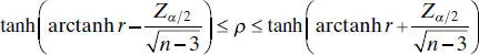

where tanh u = ( eu − e −u)/( eu + e −u).

Consider the soft drink delivery time data introduced in Chapter 1. The 25 observations on delivery time y and delivery volume x are listed in Table 2.11. The scatter diagram shown in Figure 1.1indicates a strong linear relationship between delivery time and delivery volume. The Minitab output for the simple linear regression model is in Table 2.12.