Douglas C. Montgomery - Introduction to Linear Regression Analysis
Здесь есть возможность читать онлайн «Douglas C. Montgomery - Introduction to Linear Regression Analysis» — ознакомительный отрывок электронной книги совершенно бесплатно, а после прочтения отрывка купить полную версию. В некоторых случаях можно слушать аудио, скачать через торрент в формате fb2 и присутствует краткое содержание. Жанр: unrecognised, на английском языке. Описание произведения, (предисловие) а так же отзывы посетителей доступны на портале библиотеки ЛибКат.
- Название:Introduction to Linear Regression Analysis
- Автор:
- Жанр:
- Год:неизвестен
- ISBN:нет данных
- Рейтинг книги:4 / 5. Голосов: 1
-
Избранное:Добавить в избранное
- Отзывы:
-
Ваша оценка:
Introduction to Linear Regression Analysis: краткое содержание, описание и аннотация
Предлагаем к чтению аннотацию, описание, краткое содержание или предисловие (зависит от того, что написал сам автор книги «Introduction to Linear Regression Analysis»). Если вы не нашли необходимую информацию о книге — напишите в комментариях, мы постараемся отыскать её.
New exercises and data sets New material on generalized regression techniques The inclusion of JMP software in key areas Carefully condensing the text where possible
skillfully blends theory and application in both the conventional and less common uses of regression analysis in today's cutting-edge scientific research. The text equips readers to understand the basic principles needed to apply regression model-building techniques in various fields of study, including engineering, management, and the health sciences.
Introduction to Linear Regression Analysis — читать онлайн ознакомительный отрывок
Ниже представлен текст книги, разбитый по страницам. Система сохранения места последней прочитанной страницы, позволяет с удобством читать онлайн бесплатно книгу «Introduction to Linear Regression Analysis», без необходимости каждый раз заново искать на чём Вы остановились. Поставьте закладку, и сможете в любой момент перейти на страницу, на которой закончили чтение.
Интервал:
Закладка:
(2.58b) 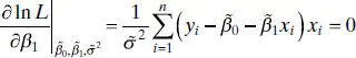
and
(2.58c) 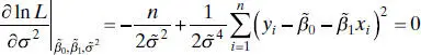
The solution to Eq. (2.58)gives the maximum-likelihood estimators:
(2.59a) 
(2.59b) 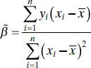
(2.59c) 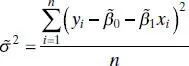
Notice that the maximum-likelihood estimators of the intercept and slope,  and
and  , are identical to the least-squares estimators of these parameters. Also,
  is a biased estimator of σ 2. The biased estimator is related to the unbiased estimator
  [ Eq. (2.19)] by
 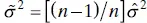 . The bias is small if n is moderately large. Generally the unbiased estimator is used.
In general, maximum-likelihood estimators have better statistical propertiesthan least-squares estimators. The maximum-likelihood estimators are unbiased(including  , which is asymptotically unbiased, or unbiased as n becomes large) and have minimum variancewhen compared to allother unbiased estimators. They are also consistent estimators(consistency is a large-sample property indicating that the estimators differ from the true parameter value by a very small amount as n becomes large), and they are a set of sufficient statistics(this implies that the estimators contain all of the “information” in the original sample of size n ). On the other hand, maximum-likelihood estimation requires more stringent statistical assumptions than the least-squares estimators. The least-squares estimators require only second-moment assumptions (assumptions about the expected value, the variances, and the covariances among the random errors). The maximum-likelihood estimators require a full distributional assumption, in this case that the random errors follow a normal distribution with the same second moments as required for the least- squares estimates. For more information on maximum-likelihood estimation in regression models, see Graybill [1961, 1976], Myers [1990], Searle [1971], and Seber [1977].
2.13 CASE WHERE THE REGRESSOR x IS RANDOM
The linear regression model that we have presented in this chapter assumes that the values of the regressor variable x are known constants. This assumption makes the confidence coefficients and type I (or type II) errors refer to repeated sampling on y at the same x levels. There are many situations in which assuming that the x ’s are fixed constants is inappropriate. For example, consider the soft drink delivery time data from Chapter 1( Figure 1.1). Since the outlets visited by the delivery person are selected at random, it is unrealistic to believe that we can control the delivery volume x . It is more reasonable to assume that both y and x are random variables.
Fortunately, under certain circumstances, all of our earlier results on parameter estimation, testing, and prediction are valid. We now discuss these situations.
2.13.1 x and y Jointly Distributed
Suppose that x and y are jointly distributed random variables but the form of this joint distribution is unknown. It can be shown that all of our previous regression results hold if the following conditions are satisfied:
1 The conditional distribution of y given x is normal with conditional mean β0 + β1x and conditional variance σ2.
2 The x’s are independent random variables whose probability distribution does not involve β0, β1, and σ2.
While all of the regression procedures are unchanged when these conditions hold, the confidence coefficients and statistical errors have a different interpretation. When the regressor is a random variable, these quantities apply to repeated sampling of ( xi , yi ) values and not to repeated sampling of yi at fixed levels of xi .
2.13.2 x and y Jointly Normally Distributed: Correlation Model
Now suppose that y and x are jointly distributed according to the bivariate normal distribution. That is,
(2.60) 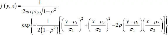
where μ 1and  the mean and variance of y , μ 2and
  the mean and variance of x , and
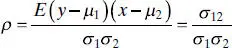
is the correlation coefficientbetween y and x . The term σ 12is the covarianceof y and x .
The conditional distributionof y for a given value of x is
(2.61) 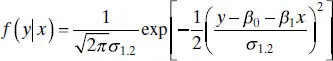
where
(2.62a) 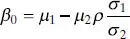
(2.62b) 
and
(2.62c) 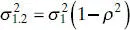
Интервал:
Закладка:
Похожие книги на «Introduction to Linear Regression Analysis»
Представляем Вашему вниманию похожие книги на «Introduction to Linear Regression Analysis» списком для выбора. Мы отобрали схожую по названию и смыслу литературу в надежде предоставить читателям больше вариантов отыскать новые, интересные, ещё непрочитанные произведения.


Обсуждение, отзывы о книге «Introduction to Linear Regression Analysis» и просто собственные мнения читателей. Оставьте ваши комментарии, напишите, что Вы думаете о произведении, его смысле или главных героях. Укажите что конкретно понравилось, а что нет, и почему Вы так считаете.