Douglas C. Montgomery - Introduction to Linear Regression Analysis
Здесь есть возможность читать онлайн «Douglas C. Montgomery - Introduction to Linear Regression Analysis» — ознакомительный отрывок электронной книги совершенно бесплатно, а после прочтения отрывка купить полную версию. В некоторых случаях можно слушать аудио, скачать через торрент в формате fb2 и присутствует краткое содержание. Жанр: unrecognised, на английском языке. Описание произведения, (предисловие) а так же отзывы посетителей доступны на портале библиотеки ЛибКат.
- Название:Introduction to Linear Regression Analysis
- Автор:
- Жанр:
- Год:неизвестен
- ISBN:нет данных
- Рейтинг книги:4 / 5. Голосов: 1
-
Избранное:Добавить в избранное
- Отзывы:
-
Ваша оценка:
Introduction to Linear Regression Analysis: краткое содержание, описание и аннотация
Предлагаем к чтению аннотацию, описание, краткое содержание или предисловие (зависит от того, что написал сам автор книги «Introduction to Linear Regression Analysis»). Если вы не нашли необходимую информацию о книге — напишите в комментариях, мы постараемся отыскать её.
New exercises and data sets New material on generalized regression techniques The inclusion of JMP software in key areas Carefully condensing the text where possible
skillfully blends theory and application in both the conventional and less common uses of regression analysis in today's cutting-edge scientific research. The text equips readers to understand the basic principles needed to apply regression model-building techniques in various fields of study, including engineering, management, and the health sciences.
Introduction to Linear Regression Analysis — читать онлайн ознакомительный отрывок
Ниже представлен текст книги, разбитый по страницам. Система сохранения места последней прочитанной страницы, позволяет с удобством читать онлайн бесплатно книгу «Introduction to Linear Regression Analysis», без необходимости каждый раз заново искать на чём Вы остановились. Поставьте закладку, и сможете в любой момент перейти на страницу, на которой закончили чтение.
Интервал:
Закладка:
The sample correlation coefficient between delivery time y and delivery volume x is
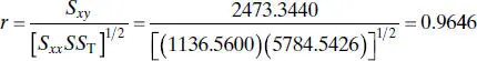
TABLE 2.11 Data Example 2.9
| Observation | Delivery Time, y | Number of Cases, x |
| 1 | 16.68 | 7 |
| 2 | 11.50 | 3 |
| 3 | 12.03 | 3 |
| 4 | 14.88 | 4 |
| 5 | 13.75 | 6 |
| 6 | 18.11 | 7 |
| 7 | 8.00 | 2 |
| 8 | 17.83 | 7 |
| 9 | 79.24 | 30 |
| 10 | 21.50 | 5 |
| 11 | 40.33 | 16 |
| 12 | 21.00 | 10 |
| 13 | 13.50 | 4 |
| 14 | 19.75 | 6 |
| 15 | 24.00 | 9 |
| 16 | 29.00 | 10 |
| 17 | 15.35 | 6 |
| 18 | 19.00 | 7 |
| 19 | 9.50 | 3 |
| 20 | 35.10 | 17 |
| 21 | 17.90 | 10 |
| 22 | 52.32 | 26 |
| 23 | 18.75 | 9 |
| 24 | 19.83 | 8 |
| 25 | 10.75 | 4 |
TABLE 2.12 MlNITAB Output for Soft Drink Delivery Time Data
Regression Analysis: Time versus Cases |
|||||
The regression equation is |
|||||
Time = 3.32 + 2.18 Cases |
|||||
Predictor |
Coef |
SE Coef |
T |
P |
|
Constant |
3.321 |
1.371 |
2.42 |
0.024 |
|
Cases |
2.1762 |
0.1240 |
17.55 |
0.000 |
|
S = 4.18140 |
R- Sq= 93.0% |
R- Sq(adj) = 92.7% |
|||
Analysis of Variance |
|||||
Source |
DF |
SS |
MS |
F |
P |
Regression |
1 |
5382.4 |
5382.4 |
307.85 |
0.000 |
Residual Error |
23 |
402.1 |
17.5 |
||
Total |
24 |
5784.5 |
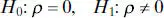
If we assume that delivery time and delivery volume are jointly normally distributed, we may test the hypotheses
using the test statistic
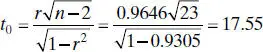
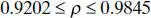
Since t 0.025,23= 2.069, we reject H 0and conclude that the correlation coefficient ρ ≠ 0. Note from the Minitab output in Table 2.12 that this is identical to the t -test statistic for H 0: β 1= 0. Finally, we may construct an approximate 95% CI on ρ from (2.72). Since arctanh r = arctanh 0.9646 = 2.0082, Eq. (2.72)becomes
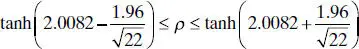
which reduces to
Although we know that delivery time and delivery volume are highly correlated, this information is of little use in predicting, for example, delivery time as a function of the number of cases of product delivered. This would require a regression model. The straight-line fit (shown graphically in Figure 1.1 b ) relating delivery time to delivery volume is
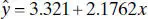
Further analysis would be required to determine if this equation is an adequate fit to the data and if it is likely to be a successful predictor.
PROBLEMS
1 2.1 Table B.1 gives data concerning the performance of the 26 National Football League teams in 1976. It is suspected that the number of yards gained rushing by opponents (x8) has an effect on the number of games won by a team (y).a. Fit a simple linear regression model relating games won y to yards gained rushing by opponents x8.b. Construct the analysis-of-variance table and test for significance of regression.c. Find a 95% CI on the slope.d. What percent of the total variability in y is explained by this model?e. Find a 95% CI on the mean number of games won if opponents’ yards rushing is limited to 2000 yards.
2 2.2 Suppose we would like to use the model developed in Problem 2.1 to predict the number of games a team will win if it can limit opponents’ yards rushing to 1800 yards. Find a point estimate of the number of games won when x8 = 1800. Find a 90% prediction interval on the number of games won.
3 2.3 Table B.2 presents data collected during a solar energy project at Georgia Tech.a. Fit a simple linear regression model relating total heat flux y (kilowatts) to the radial deflection of the deflected rays x4 (milliradians).b. Construct the analysis-of-variance table and test for significance of regression.c. Find a 99% CI on the slope.d. Calculate R2.e. Find a 95% CI on the mean heat flux when the radial deflection is 16.5 milliradians.
4 2.4 Table B.3 presents data on the gasoline mileage performance of 32 different automobiles.a. Fit a simple linear regression model relating gasoline mileage y (miles per gallon) to engine displacement xl (cubic inches).b. Construct the analysis-of-variance table and test for significance of regression.c. What percent of the total variability in gasoline mileage is accounted for by the linear relationship with engine displacement?d. Find a 95% CI on the mean gasoline mileage if the engine displacement is 275 in.3e. Suppose that we wish to predict the gasoline mileage obtained from a car with a 275-in.3 engine. Give a point estimate of mileage. Find a 95% prediction interval on the mileage.f. Compare the two intervals obtained in parts d and e. Explain the difference between them. Which one is wider, and why?
5 2.5 Consider the gasoline mileage data in Table B.3. Repeat Problem 2.4 (parts a, b, and c) using vehicle weight x10 as the regressor variable. Based on a comparison of the two models, can you conclude that x1 is a better choice of regressor than x10?
6 2.6 Table B.4 presents data for 27 houses sold in Erie, Pennsylvania.a. Fit a simple linear regression model relating selling price of the house to the current taxes (x1).b. Test for significance of regression.c. What percent of the total variability in selling price is explained by this model?d. Find a 95% CI on β1.e. Find a 95% CI on the mean selling price of a house for which the current taxes are $750.
Читать дальшеИнтервал:
Закладка:
Похожие книги на «Introduction to Linear Regression Analysis»
Представляем Вашему вниманию похожие книги на «Introduction to Linear Regression Analysis» списком для выбора. Мы отобрали схожую по названию и смыслу литературу в надежде предоставить читателям больше вариантов отыскать новые, интересные, ещё непрочитанные произведения.


Обсуждение, отзывы о книге «Introduction to Linear Regression Analysis» и просто собственные мнения читателей. Оставьте ваши комментарии, напишите, что Вы думаете о произведении, его смысле или главных героях. Укажите что конкретно понравилось, а что нет, и почему Вы так считаете.