Douglas C. Montgomery - Introduction to Linear Regression Analysis
Здесь есть возможность читать онлайн «Douglas C. Montgomery - Introduction to Linear Regression Analysis» — ознакомительный отрывок электронной книги совершенно бесплатно, а после прочтения отрывка купить полную версию. В некоторых случаях можно слушать аудио, скачать через торрент в формате fb2 и присутствует краткое содержание. Жанр: unrecognised, на английском языке. Описание произведения, (предисловие) а так же отзывы посетителей доступны на портале библиотеки ЛибКат.
- Название:Introduction to Linear Regression Analysis
- Автор:
- Жанр:
- Год:неизвестен
- ISBN:нет данных
- Рейтинг книги:4 / 5. Голосов: 1
-
Избранное:Добавить в избранное
- Отзывы:
-
Ваша оценка:
Introduction to Linear Regression Analysis: краткое содержание, описание и аннотация
Предлагаем к чтению аннотацию, описание, краткое содержание или предисловие (зависит от того, что написал сам автор книги «Introduction to Linear Regression Analysis»). Если вы не нашли необходимую информацию о книге — напишите в комментариях, мы постараемся отыскать её.
New exercises and data sets New material on generalized regression techniques The inclusion of JMP software in key areas Carefully condensing the text where possible
skillfully blends theory and application in both the conventional and less common uses of regression analysis in today's cutting-edge scientific research. The text equips readers to understand the basic principles needed to apply regression model-building techniques in various fields of study, including engineering, management, and the health sciences.
Introduction to Linear Regression Analysis — читать онлайн ознакомительный отрывок
Ниже представлен текст книги, разбитый по страницам. Система сохранения места последней прочитанной страницы, позволяет с удобством читать онлайн бесплатно книгу «Introduction to Linear Regression Analysis», без необходимости каждый раз заново искать на чём Вы остановились. Поставьте закладку, и сможете в любой момент перейти на страницу, на которой закончили чтение.
Интервал:
Закладка:
There are alternative ways to define R 2for the no-intercept model. One possibility is
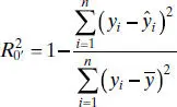
However, in cases where  is large,
  can be negative. We prefer to use MS Resas a basis of comparison between intercept and no-intercept regression models. A nice article on regression models with no intercept term is Hahn [1979].
Example 2.8 The Shelf-Stocking Data
The time required for a merchandiser to stock a grocery store shelf with a soft drink product as well as the number of cases of product stocked is shown in Table 2.10. The scatter diagram shown in Figure 2.14suggests that a straight line passing through the origin could be used to express the relationship between time and the number of cases stocked. Furthermore, since if the number of cases x = 0, then shelf stocking time y = 0, this model seems intuitively reasonable. Note also that the range of x is close to the origin.
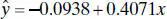
The slope in the no-intercept model is computed from Eq. (2.50)as
Therefore, the fitted equation is

This regression line is shown in Figure 2.15. The residual mean square for this model is MS Res= 0.0893 and  . Furthermore, the t statistic for testing H 0: β 1= 0 is t 0= 91.13, for which the P value is 8.02 × 10 −21. These summary statistics do not reveal any startling inadequacy in the no-intercept model.
We may also fit the intercept model to the data for comparative purposes. This results in
The t statistic for testing H 0: β 0= 0 is t 0= −0.65, which is not significant, implying that the no-intercept model may provide a superior fit. The residual mean square for the intercept model is MS Res= 0.0931 and R 2= 0.9997. Since MS Resfor the no-intercept model is smaller than MS Resfor the intercept model, we conclude that the no-intercept model is superior. As noted previously, the R 2statistics are not directly comparable.
TABLE 2.10 Shelf-Stocking Data for Example 2.8
| Times, y (minutes) | Cases Stocked, x |
| 10.15 | 25 |
| 2.96 | 6 |
| 3.00 | 8 |
| 6.88 | 17 |
| 0.28 | 2 |
| 5.06 | 13 |
| 9.14 | 23 |
| 11.86 | 30 |
| 11.69 | 28 |
| 6.04 | 14 |
| 7.57 | 19 |
| 1.74 | 4 |
| 9.38 | 24 |
| 0.16 | 1 |
| 1.84 | 5 |
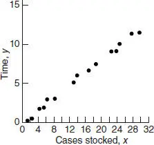
Figure 2.14 Scatter diagram of shelf-stocking data.
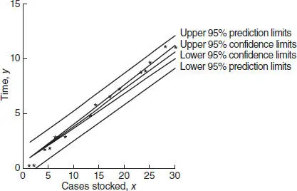
Figure 2.15 The confidence and prediction bands for the shelf-stocing data.
Figure 2.15also shows the 95% confidence interval or E ( y | x 0) computed from Eq. (2.54)and the 95% prediction interval on a single future observation y 0at x = x 0computed from Eq. (2.55). Notice that the length of the confidence interval at x 0= 0 is zero.
SAS handles the no-intercept case. For this situation, the model statement follows:
model time = cases/noint
2.12 ESTIMATION BY MAXIMUM LIKELIHOOD
The method of least squares can be used to estimate the parameters in a linear regression model regardless of the form of the distribution of the errors ε. Least squares produces best linear unbiased estimators of β 0and β 1. Other statistical procedures, such as hypothesis testing and CI construction, assume that the errors are normally distributed. If the form of the distribution of the errors is known, an alternative method of parameter estimation, the method of maximum likelihood, can be used.
Consider the data ( yi , xi ), i = 1, 2, …, n . If we assume that the errors in the regression model are NID(0, σ 2), then the observations yi in this sample are normally and independently distributed random variables with mean β 0+ β 1 xi and variance σ 2. The likelihood function is found from the joint distribution of the observations. If we consider this joint distribution with the observations given and the parameters β 0, β 1, and σ 2unknown constants, we have the likelihood function. For the simple linear regression model with normal errors, the likelihood functionis
(2.56) 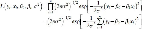
The maximum-likelihood estimators are the parameter values, say  ,
,  , and
, and  , that maximize L , or equivalently, ln L . Thus,
(2.57) 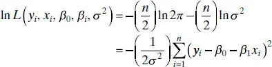
and the maximum-likelihood estimators  ,
,  , and
, and  must satisfy
(2.58a) 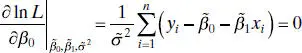
Интервал:
Закладка:
Похожие книги на «Introduction to Linear Regression Analysis»
Представляем Вашему вниманию похожие книги на «Introduction to Linear Regression Analysis» списком для выбора. Мы отобрали схожую по названию и смыслу литературу в надежде предоставить читателям больше вариантов отыскать новые, интересные, ещё непрочитанные произведения.


Обсуждение, отзывы о книге «Introduction to Linear Regression Analysis» и просто собственные мнения читателей. Оставьте ваши комментарии, напишите, что Вы думаете о произведении, его смысле или главных героях. Укажите что конкретно понравилось, а что нет, и почему Вы так считаете.