Douglas C. Montgomery - Introduction to Linear Regression Analysis

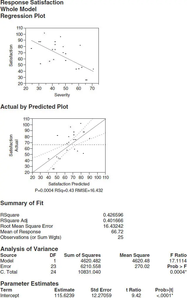
Figure 2.7 JMP output for the simple linear regression model for the patient satisfaction data.

Low values for R 2occur occasionally in practice. The model is significant, there are no obvious problems with assumptions or other indications of model inadequacy, but the proportion of variability explained by the model is low. Now this is not an entirely disastrous situation. There are many situations where explaining 30 to 40% of the variability in y with a single predictor provides information of considerable value to the analyst. Sometimes, a low value of R 2results from having a lot of variability in the measurements of the response due to perhaps the type of measuring instrument being used, or the skill of the person making the measurements. Here the variability in the response probably arises because the response is an expression of opinion, which can be very subjective. Also, the measurements are taken on human patients, and there can be considerably variability both within people and between people. Sometimes, a low value of R 2is a result of a poorly specified model. In these cases the model can often be improved by the addition of one or more predictor or regressor variables. We see in Chapter 3that the addition of another regressor results in considerable improvement of this model.

Part of the never-ending debate about what makes a winning baseball team is the theory that a team cannot win consistently without good pitching. Baseball is a sport deeply rooted in analytics and there is an ever-growing body of data available. Major league baseball now has a system in all stadiums that includes cameras and other sensors to collect data on every pitch, including pitch speed, player positions, launch angle for balls hit in the air, and so forth. Table B.22 contains a summary of performance for 2016 for all National and American League baseball teams. The response variable is the number of games won and among the various statistics listed is the team earned run average (ERA), a standard measure of pitching performance, with low values of team ERA generally attributed to an outstanding pitching staff. Figure 2.8is the JMP output from fitting a linear regression model to wins versus the ERA data. The plots of wins versus ERA and actual versus predicted show that there is definitely a linear relationship between these variables. The model is significant and it seems that one point of team ERA is equivalent to about 18.6 wins. JMP also produces a plot of residuals versus the predicted number of wins. Residual plots such as this are useful in assessing model adequacy. We will discuss this in detail later but this plot indicates that there is no structure in the relationship between the residuals and the predicted number of wins. This is one indication that the model fit is satisfactory. However, the model only explains about 63% of the variability in the response. While this is not bad, it does suggest that there may be other useful explanatory variables.

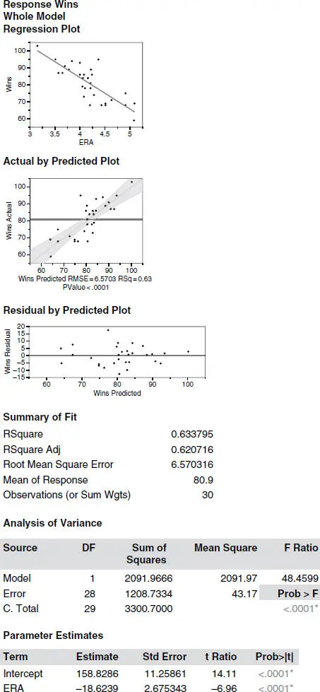
Figure 2.8 JMP output for the model relating team wins to team ERA for the 2016 baseball season.

The purpose of this section is to introduce readers to SAS and to R. Appendix Dgives more details about using SAS, including how to import data from both text and EXCEL files. Appendix Eintroduces the R statistical software package. R is becoming increasingly popular since it is free over the Internet.

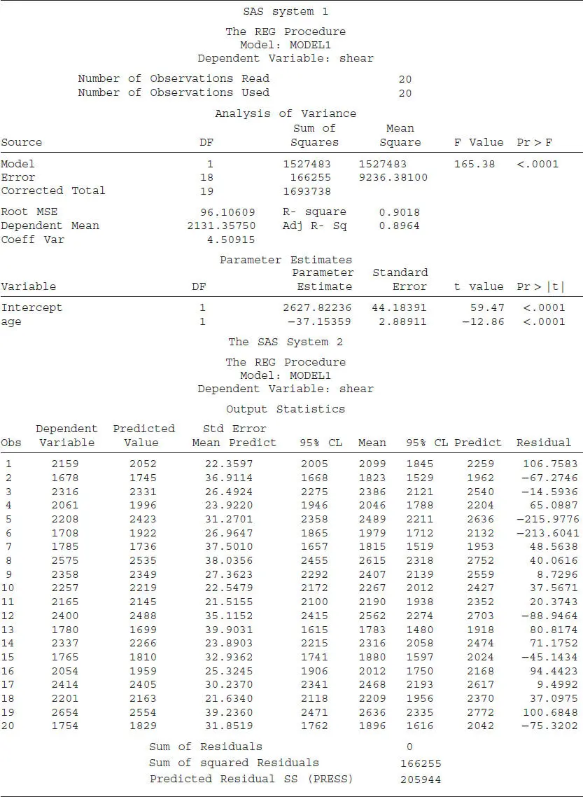
Table 2.7 gives the SAS source code to analyze the rocket propellant data that we have been analyzing throughout this chapter. Appendix Dprovides detail explaining how to enter the data into SAS. The statement PROC REG tells the software that we wish to perform an ordinary least-squares linear regression analysis. The “model” statement specifies the specific model and tells the software which analyses to perform. The variable name to the left of the equal sign is the response. The variables to the right of the equal sign but before the solidus are the regressors. The information after the solidus specifies additional analyses. By default, SAS prints the analysis-of-variance table and the tests on the individual coefficients. In this case, we have specified three options: “p” asks SAS to print the predicted values, “clm” (which stands for confidence limit, mean) asks SAS to print the confidence band, and “cli” (which stands for confidence limit, individual observations) asks SAS to print the prediction band.

Table 2.8 gives the SAS output for this analysis. PROC REG always produces the analysis-of-variance table and the information on the parameter estimates. The “p clm cli” options on the model statement produced the remainder of the output file.

TABLE 2.7 SAS Code for Rocket Propellant Data

TABLE 2.8 SAS Output for Analysis of Rocket Propellant Data.

SAS also produces a log file that provides a brief summary of the SAS session. The log file is almost essential for debugging SAS code. Appendix Dprovides more details about this file.

R is a popular statistical software package, primarily because it is freely available at www.r-project.org. An easier-to-use version of R is R Commander. R itself is a high-level programming language. Most of its commands are prewritten functions. It does have the ability to run loops and call other routines, for example, in C. Since it is primarily a programming language, it often presents challenges to novice users. The purpose of this section is to introduce the reader as to how to use R to analyze simple linear regression data sets.