
– There are two possible cases when K ≠ M.- Consider the case where K < M, an example of the mapping here could beas an example only, and- for the case of K > M, an example of the mapping here could beagain just an example.
The K interarrival times can each be written as PH distribution ( α ( k ), T ( k )), where k = 1,2, ..., K . Hence the resulting interarrival time, which is a function of the service time, is a PH distribution represented by  where
where

where α= [ α (1), α (2), ∙∙∙ , α (k)] and the operator * is the Khatri-Rao (K-R) product (Khatri and Rao 1968) , and here we have

In applying K-R operator, here the first vector ψ is partitioned into K , 1 × 1 vectors, i.e. into scalars in order to properly apply the K-R operator.
This is better illustrated with an example.
Example
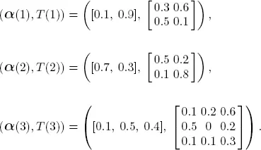
Consider a case of a service time S with  i.e. M = 4 . Let K = 3 , with the three interarrival PH distributions given as ( α( k ), T ( k )), k =
  as an example.
Then we have a system with service time distribution vector given as s= [ s 1, s 2, s 3, s 4] and interarrival time distribution given as a PH with

Numerical examples
Let s=[0.1, 0.3, 0.4, 0.2] and
suppose we select three mappings of s with 

 We can then generate two PH distributions that are both dependent on s, but with different mappings with both having the same T given as follows

but different  .
.
Let Aj be the interarrival times for the j th mapping and  . Table 1.2summarizes the results.
Table 1.2. Complementary Cumulative distributions of interarrival times
| k |
1 |
2 |
3 |
4 |
5 |
6 |
7 |
8 |
9 |
| P1(k) |
0.6490 |
0.4886 |
0.3311 |
0.2382 |
0.1704 |
0.1246 |
0.0919 |
0.688 |
0.0522 |
| P2(k) |
0.7110 |
0.5526 |
0.4225 |
0.3361 |
0.2705 |
0.2210 |
0.1823 |
0.1516 |
0.1268 |
| P3(k) |
0.6740 |
0.5128 |
0.3657 |
0.2751 |
0.2084 |
0.1613 |
0.1265 |
0.1006 |
0.0810 |
In future works, we study how the different arrangements of s affect the features and distribution and moments of the interarrival times. This can be used to show how one can control the arrival process and hence the queue performance by using different selections of the vector s.
1.4.2. A queueing model with interarrival times dependent on service times
Consider a single-server queue with service times distribution vector, given as sof M dimension and K independent interarrival times, from which a customer’s next interarrival is selected based on the service time experienced by customers. It is clear that the true interarrival times is Markovian Arrival Process (MAP), which is constructed from the K interarrival times and the probability vector ψ of dimension K that was created by mapping service distribution as shown in section 1.4.1. The PH representation of interarrival times has κ = k 1+ k 2+ ... + kK , where kj is the number of phases of the jth interarrival time. We let the service times be represented by an elapsed time PH distribution with representation ( β , B ) of order M . Also let b = 1 – B 1.
At time n = 0, 1, 2, 3, ∙∙∙, let Xn be the number of customers in the system, Y nthe phase of arrival and J nthe phase of the ongoing service. The stochastic process {( Xn,Jn,Yn ), n ≥ 0} is a DTMC with transition matrix P given as

where

This Markov chain is a simple Quasi-Birth-Death (QBD), which can be analyzed using the matrix-analytical methods for discrete time queues (Neuts 1981; Alfa2016).
If this system is stable, which we will assume it is, then there is a unique probability vector  for which we have

Further, we have  and
and 
Читать дальше


 where
where

 i.e. M = 4 . Let K = 3 , with the three interarrival PH distributions given as ( α( k ), T ( k )), k =
  as an example.


 We can then generate two PH distributions that are both dependent on s, but with different mappings with both having the same T given as follows
 .
. . Table 1.2summarizes the results.

 for which we have
 and
and 


