Nikolaos Limnios - Queueing Theory 1

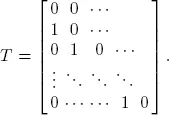
It was shown in Alfa (2004) that any discrete distribution, with finite support, can be represented by PH distribution with elapsed time or remaining time format. For example, consider the interarrival Aand let . In the elapsed time format, the matrix T has only its superdiagonal elements that are non-zero and every other element is zero, and the vector α= [1, 0, 0, ∙∙∙ , ], and the matrix T is written as

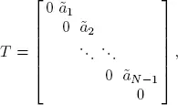
where

For the remaining time representation, the vector is the vector of the discrete distribution and the matrix T is written as

Consider a PH/PH/1 system with interarrival times and service times that are represented by ( α ,T ) and ( β, B ), respectively, with means given as a –1and b –1. Note that a –1= α( I – T ) –1 1and b –1= β ( I – B ) –1 1. At time t ≥ 0, let Xt be the number of items in the system, Yt the phase of interarrival times and Z tthe phase of the ongoing service. It is straightforward to see that ( Xt, Yt, Zt ), t ≥ 0, is a DTMC with transition matrix P given as

where

and where ⊗ is the Kronecker product. For two matrices U of order n × m and V of order r × k , the product U ⊗ W is a matrix of order nr × mk (for more details, see Graham 1981).

It is well-known in the literature that for a stable PH/PH/1 system there is a matrix R, with spectral radius less than 1, which is the minimal non-negative solution to and the stationary distribution of the DTMC, which is given as can be obtained through the matrix-geometric theorem (Neuts 1981) as

after appropriately obtaining the boundary solution [ x 0, x 1]. For more details, see Alfa (2016).

The idea of the Geo/Geo/1 system discussed in section 1.2can be extended to the PH/PH/1, but requires a more involved representation and analysis. Consider the case where ( α,T ) depends on ( β, B ). The dependence can be captured by letting

with the condition that

We see that the case of the Geo/Geo/1 is a special case where ( β, B ) = (1, b ), hence . several functional forms of α= gα ( β ), and T = fT ( B ) can be studied, but are beyond the scope of this chapter. However, a small example of a representation is presented as an illustration. Consider a simple case with T and B having the same size, i.e. n × n . Define a doubly stochastic matrix V of order n × n . We can select

provided

Even though this system is more complicated to analyze compared to the Geo/Geo/1 case, the idea is exactly the same and it can be studied numerically.

Next we consider a model in which there is a general service time distribution; however, there are several interarrival time distributions and the selection of the next interarrival time distribution depends on the service time distribution.

We consider the case where the service times are independent and the interarrival times depend on the distribution of the service times, and not just one parameter such as the mean:

– let the service time, S, be of a general renewal type in discrete time with finite support. Let Let us write s = [s1, s2, ∙∙∙ , sM];

– let there be K interarrival times with the selection of the interarrival time depending on the service time. Let be the interarrival time between the nth and the st customer if the kth interarrival is selected. Let

– by the results in Alfa (2004), we can represent each of the K interarrival times by discrete PH distribution and in this case chose the remaining time approach. Let (α(k), T(k)) be the PH representation for the kth interarrival time distribution of dimension .

Next we define some parameters that will be used to relate the interarrival times to the service times.

Define a K × M matrix EKM such that its elements have values of 0 or 1 and in addition

– for K ≥ M, we require that and ;

– for K ≤ M, we require that , and

Next we define a stochastic vector ψ =[ ψ 1, ψ 2, ... , ψ K], which is a function of s, i.e. ψ = f( s), where f : R M→ R K. We give some very simple examples of this type of mapping.

– Consider the case when K = M . A simple mapping of f could be ψ i= s i, ∀ i, i.e. ψ = s. Another possible example could be . Finally, we could generate ψ from susing any argument possible, as long as ψ depends on s. For this simple example alone, there are K! ways of generating the mapping by rearranging the elements of ψ , if we keep the values of si unchanged, e.g.