Anand K. Verma - Introduction To Modern Planar Transmission Lines
Здесь есть возможность читать онлайн «Anand K. Verma - Introduction To Modern Planar Transmission Lines» — ознакомительный отрывок электронной книги совершенно бесплатно, а после прочтения отрывка купить полную версию. В некоторых случаях можно слушать аудио, скачать через торрент в формате fb2 и присутствует краткое содержание. Жанр: unrecognised, на английском языке. Описание произведения, (предисловие) а так же отзывы посетителей доступны на портале библиотеки ЛибКат.
- Название:Introduction To Modern Planar Transmission Lines
- Автор:
- Жанр:
- Год:неизвестен
- ISBN:нет данных
- Рейтинг книги:4 / 5. Голосов: 1
-
Избранное:Добавить в избранное
- Отзывы:
-
Ваша оценка:
Introduction To Modern Planar Transmission Lines: краткое содержание, описание и аннотация
Предлагаем к чтению аннотацию, описание, краткое содержание или предисловие (зависит от того, что написал сам автор книги «Introduction To Modern Planar Transmission Lines»). Если вы не нашли необходимую информацию о книге — напишите в комментариях, мы постараемся отыскать её.
rovides a comprehensive discussion of planar transmission lines and their applications, focusing on physical understanding, analytical approach, and circuit models
Planar transmission lines form the core of the modern high-frequency communication, computer, and other related technology. This advanced text gives a complete overview of the technology and acts as a comprehensive tool for radio frequency (RF) engineers that reflects a linear discussion of the subject from fundamentals to more complex arguments.
Introduction to Modern Planar Transmission Lines: Physical, Analytical, and Circuit Models Approach Emphasizes modeling using physical concepts, circuit-models, closed-form expressions, and full derivation of a large number of expressions Explains advanced mathematical treatment, such as the variation method, conformal mapping method, and SDA Connects each section of the text with forward and backward cross-referencing to aid in personalized self-study
is an ideal book for senior undergraduate and graduate students of the subject. It will also appeal to new researchers with the inter-disciplinary background, as well as to engineers and professionals in industries utilizing RF/microwave technologies.
Introduction To Modern Planar Transmission Lines — читать онлайн ознакомительный отрывок
Ниже представлен текст книги, разбитый по страницам. Система сохранения места последней прочитанной страницы, позволяет с удобством читать онлайн бесплатно книгу «Introduction To Modern Planar Transmission Lines», без необходимости каждый раз заново искать на чём Вы остановились. Поставьте закладку, и сможете в любой момент перейти на страницу, на которой закончили чтение.
Интервал:
Закладка:
The field decreases by a factor e −αx ,whereas the wave travels through a lossy medium. If the wave travels a distance x = δ = 1/α, known as the skin depth, the field is decreased by 1/e of its initial strength, i.e. approximately 37% of its initial field strength. However, the power decreases at a faster rate, i.e. by the factor e −2αx. If the initial power density is S 0, the power density at distance x is
(4.5.44) 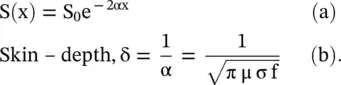
The attenuation constant α in the above equation is used from equation (4.5.35b). The power loss of wave traveling a distance x is computed after computing the power loss at unit distance x = 1m:
(4.5.45) 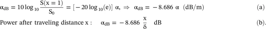
In the above equation, the value of e is 2.71828. The power loss is about 9 dB per skin‐depth. The attenuation constant α of a lossy medium is defined by equation (4.5.44a)as follows:
(4.5.46) 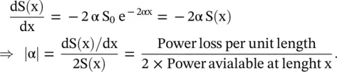
4.6 Polarization of EM‐waves
The uniform plane wave in the unbounded medium is the TEM‐type wave. The monochromatic EM‐wave is characterized by amplitude , phase , and polarization states . The microwave to optical wave devices can appropriately manipulate these characteristics to steer the EM‐waves in the desired direction with shaped wavefront. The modern metasurfaces, discussed in sections (22.5) and (22.6) of chapter 22, can achieve such controls on the reflected and transmitted waves.
In general, both  and
and  fields have two orthogonal field components in a plane normal to the direction of propagation, the x‐direction, as shown in Fig. (4.9a and b). The field components are in the (y‐z)‐plane. For the TEM mode, it is possible to get either (E y, H z) or (E z, H y) pair of fields. Both pairs of field components can also exist. The orientation of the electric field component and the movement of the tip of the resultant E‐field determine the polarization of the EM‐wave. Thus, the (E y, H z) pair of the EM‐wave is called a y ‐polarized wave, as only the E ycomponent of wave exists. The (E z, H y) pair of the EM‐wave is called the z‐polarized wave . The (y‐z)‐plane is known as the plane of polarization . It is normal to the direction of propagation, i.e. the x‐axis. Both these polarizations are linear polarization .
Figure (4.9a and c)show that for the EM‐wave propagating in the x‐direction, the tip of the E yfield component moves along the y‐axis from +E 0to 0 to −E 0. The movement and rotation of the tip of the  ‐vector could be seen using the instantaneous
  ‐vector of the wave propagating in the x‐direction. In Fig. (4.9c), the path of the tip of the E y‐field vector, in the plane of polarization, traces a line with respect to time. The linear trace demonstrates the vertical linear polarization . However, if both E yand E zfield components are present, any of the three kinds of wave polarizations can be obtained: (i) linear polarization, (ii) circular polarization, and (iii) elliptical polarization . These polarizations are shown in Fig. (4.10a–c). The type of wave polarization depends upon the magnitude and the relative phase of the orthogonal E yand E zfield components. The polarization states are briefly discussed below. Finally, the Jones vector and Jones matrix descriptions are summarized to describe elegantly the polarization states and their control by the polarizing devices.
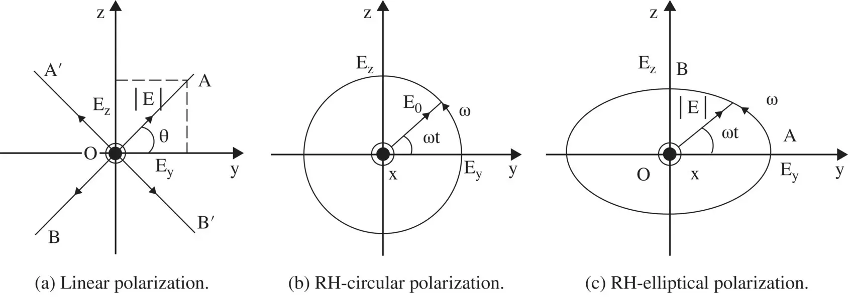
Figure 4.10 Type of polarizations.
4.6.1 Linear Polarization
Figure (4.10a)shows E yand E zfield components of the EM‐wave propagating in the x‐direction. The E‐electric field vector in the (y‐z)‐plane could be written in the phasor form as follows:
(4.6.1) 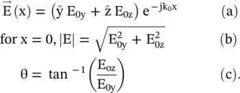
The e jωttime‐harmonic factor is suppressed in the above equation (4.6.1a). Equation (4.6.1b)shows the magnitude of the E‐field, and equation (4.6.1c)computes its inclination with respect to the y‐axis. For y‐polarized wave, E 0z= 0, and for the z‐polarized wave, E 0y= 0. In general, the field components E 0yand E 0zare complex quantities. For the in‐phase field components, these are expressed as E 0y=|E 0y| e jφand E 0z=|E 0z| e jφ. The instantaneous field components are considered to trace the movement of the tip of the  ‐vector:
(4.6.2) 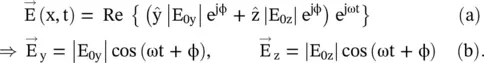
In the above equations, both field components have an identical phase (ωt + φ). Figure (4.10a)shows the slant or inclined linearly polarized wave with the in‐phase E yand E zcomponents. The tip of the electric vector (  ) moves along line A‐O‐B with respect to time. However, the slant angle θ does not change with time. If both the E‐field components are either in‐phase (A − O − B) or out of phase (A /− O − B /) and have the same magnitude, i.e. E 0y= E 0z= E 0, the corresponding inclination angle of the linear polarization trace, with respect to the y‐axis, is θ = 45° and 135°, respectively. For the linear polarization, the total E‐field given by equation (4.6.1a)could also be written as follows:
(4.6.3) 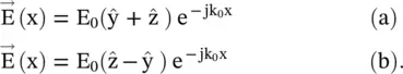
4.6.2 Circular Polarization
The circular polarization, shown in Fig. (4.10b), is obtained for two orthogonal field components of equal magnitude, and phase in quadrature. So, to get the circular polarization, two electric field components oscillate at the same frequency and meet the following conditions:
Equal amplitude: The magnitudes of Ey and Ez are equal, i.e. |E0y| = |E0z| = E0.
Space quadrature: The Ey and Ez field components are normal to each other.
Time (phase) quadrature: The phase difference between the Ey and Ez field components are (φ = ± 90°), i.e. E0y = E0, and E0z = E0e±π/2 = ± j E0.
Читать дальшеИнтервал:
Закладка:
Похожие книги на «Introduction To Modern Planar Transmission Lines»
Представляем Вашему вниманию похожие книги на «Introduction To Modern Planar Transmission Lines» списком для выбора. Мы отобрали схожую по названию и смыслу литературу в надежде предоставить читателям больше вариантов отыскать новые, интересные, ещё непрочитанные произведения.


Обсуждение, отзывы о книге «Introduction To Modern Planar Transmission Lines» и просто собственные мнения читателей. Оставьте ваши комментарии, напишите, что Вы думаете о произведении, его смысле или главных героях. Укажите что конкретно понравилось, а что нет, и почему Вы так считаете.