Anand K. Verma - Introduction To Modern Planar Transmission Lines

Figure (4.11)shows that the polarizing device could be described by a 2 × 2 transfer matrix, i.e. the Jones matrix [J]. It relates the output of the device to its input. The input could be the incident wave at certain slab/surface, acting as a polarizing device, and the output could be the transmission or reflection of the waves.

(4.6.13)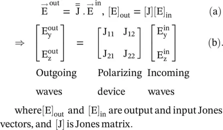

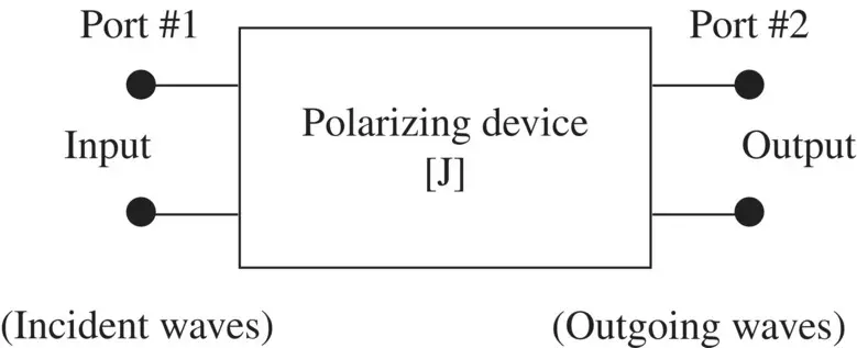
Figure 4.11 Polarizing device described by Jones matrix.

The Jones matrix elements are interpreted in the terms of the co‐polarized and cross‐polarized outgoing waves after transmission/reflection from a slab/surface:

(4.6.14)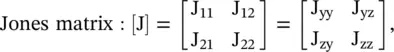

where J yyand J zzare responsible for the co‐polarized outgoing waves, and J yzand J zyaccount for the presence of cross‐polarized waves at the output. The co‐polarized output waves have the same polarization as that of the incident input waves. Whereas, the cross‐polarized output waves have orthogonal polarization with respect to the polarization of the incident input waves.

A linear polarizer allows the transmission of the incoming wave only along the transmission axis of the polarizer and blocks the transmission of the orthogonal polarizations. Jones matrices of the linear polarizers are summarized below:

(4.6.15)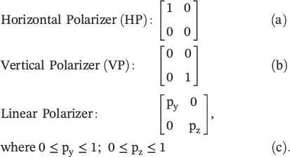

For instance, at an inclination angle θ = 45° ,the linearly polarized wave, given by Jones vector of equation (4.6.12c), is incident on the horizontal polarizer. The polarizer will provide a horizontally polarized wave given by equation (4.6.12a). It could be examined with the help of equation (4.6.13).

Figure (4.12)shows the (y‐z)‐coordinate system and also the (e 1‐e 2) ‐coordinate system rotated at an angle θ with respect to the y‐axis. The original polarizer , located in the (y‐z)‐coordinate system is described by the Jones matrix [J]; and the rotated polarizer at an angle θ is described as the rotated Jones matrix [J rot(θ)]. The rotated polarizer is located in the (e 1‐e 2) coordinate system. The relation between the Jones matrix [J] of unrotated polarizer and Jones matrix [J rot(θ)] of the rotated polarizer is obtained by the coordinate transformation through the rotation Jones matrix [R θ(θ)] and the inverse rotation Jones matrix [R θ(θ)] −1= [R θ(−θ)].

Figure (4.12)shows that the unit vectors of two coordinate systems are related through the following transformations:

(4.6.16)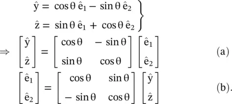

The following rotation Jones matrix [R θ(θ)] and its inverse [R θ(−θ)] can be defined from the above relations that could be useful to transform the vectors from one co‐ordinated system to another:

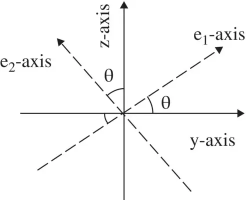
Figure 4.12 The (y–z) and rotated (e 1–e 2) Coordinate systems.

(4.6.17)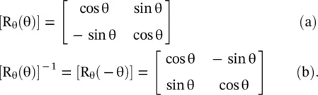

The above rotation matrices are used to transform both the Jones vector and the Jones matrix from one to another coordinate system. The Jones matrix concept is applied to the polarizing system in two steps:

The rotation Jones matrix [R θ(θ)] transforms the vector components from the rotated (e 1‐e 2) coordinate system to the (y‐z) Cartesian coordinate system. Whereas the inverse rotation Jones matrix [R θ(−θ)] transforms the vector components from the (y‐z) Cartesian coordinate system back to the rotated (e 1‐e 2) coordinate system.

To perform the transformation of the E‐vector components from one to another coordinate system using a polarizer, the Jones matrix describing the polarizer has to be transformed from one to another coordinated system. Thus, the above relations transform the Jones matrix [J] = [J] Carof a linear polarizer, given by equation (4.6.14)in the Cartesian (y‐z) coordinate system, to the Jones matrix [J rot(θ)] = [J] eof the polarizer in the rotated (e 1‐e 2) coordinate system.

The input/output relations of the E‐field in both coordinate systems are expressed in terms of their respective Jones matrices:

(4.6.18)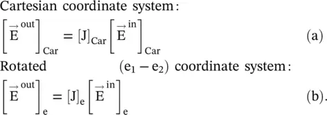

In the above expression, subscript “Car.” with Jones matric stands for the (y‐z) Cartesian coordinate system; and the subscript “e” with Jones matric stands for the general (e 1‐e 2) coordinate system. In the present case, it is the anticlockwise rotated Cartesian system, as shown in Fig. (4.12).

Using the rotation Jones matrices of equation (4.6.17a), the input and output E‐field vectors could be transformed from the rotated (e 1‐e 2) coordinate system to the Cartesian (y‐z) coordinate system:

(4.6.19)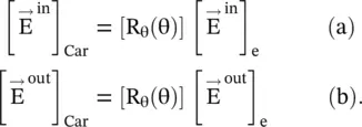

On substituting the above equations in equation (4.6.18a), the following expression is obtained:

(4.6.20)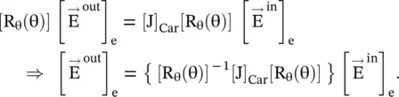

On comparing the above equations against equation (4.6.18b), we get the transformed Jones matrix [J] eof the rotated polarizer in the (e 1‐e 2) coordinate system from the Jones matrix [J] Carof the original polarizer in the Cartesian (y‐z) coordinate system:

(4.6.21)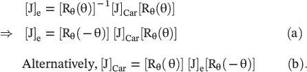

The transformation (4.6.21b)transforms the Jones matrix [J] edescribing a polarizer in the rotated (e 1‐e 2) coordinate system to the Jones matrix [J] Carin the Cartesian coordinate system. The transformation equation (4.6.21b)is obtained by matrix manipulation. However, it could also be obtained independently, as it is done for equation (4.6.21a).

The use of the coordinate transformation for the polarizer is illustrated below by a few illustrative simple examples. Application of Jones matrix to the more complex polarizing system is available in the reference [B.30].