Anand K. Verma - Introduction To Modern Planar Transmission Lines

(3.3.13)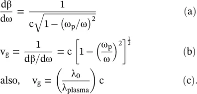

The group velocity is less than the velocity of the EM‐wave in the free space, v g≤ c. In summary, the plasma forms a fast‐wave normal dispersive medium that supports the forward wave having the same direction for both the phase and group velocities. Equations (3.3.8d)and (3.3.13c)for the wave propagation in a nonmagnetized plasma with μ = μ 0, ε 0and v = c show that the phase and group velocities are related through the following expression:

(3.3.14)

In equation (3.3.14), the general isotropic medium supports EM‐wave propagation with velocity .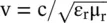

A more general relation between the phase and group velocities could be obtained. In the dispersive medium, phase velocity (v p) is a function of frequency; therefore,

(3.3.15)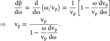

Figure (3.26a and b)show the dispersive behaviors of the phase velocity (v p) and propagation constant (β). The expression for the group velocity in a dispersive medium, i.e. a medium with frequency‐dependent refractive index 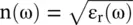, can be rewritten as follows:

(3.3.16)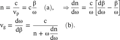

In equation (3.3.16), c is the velocity of EM‐wave in free space. The cases of dispersion are considered below:

Case‐I: . It is the no dispersion case. In this case, the above equation provides vg = vp. Figure (3.26a)shows that the phase velocity in a nondispersive medium remains unchanged with angular frequency. Figure (3.26b)shows that the propagation constant (β) is a linear function of angular frequency (ω). The free space is one such medium.

Case‐II: . It is the case of normal, i.e. the positive dispersion. Figure (3.26b)indicates that the slope of the propagation constant β in the normal dispersive medium increases nonlinearly with angular frequency ω. Therefore, the phase velocity decreases with angular frequency, i.e. dvp/dω is negative. It is shown in Fig (3.26a). For this case, equations (3.3.15)and (3.3.16)show that vg < vp. It is the case applicable to a dispersive microstrip line. Figure 3.26 Nature of dispersion on (ω − β) the diagram.

Case‐III: . It is the case of the anomalous (abnormal), i.e. the negative dispersion. The propagation constant β of such an anomalous dispersive medium increases nonlinearly with angular frequency ω. However, on the (ω − β) diagram, shown in Fig (3.26b), its value is below the dispersionless medium of the case‐I. The slope of the propagation constant β, in the nonlinear region, decreases with an increase in frequency ω, i.e. dn/dω < 0. Figure (3.26a)shows that the phase velocity increases with angular frequency, i.e. dvp/dω is positive. Equations (3.3.15)and (3.3.16)show that vg > vp. However, the group velocity in an anomalous dispersive medium is not the velocity of energy transportation. This case is applicable to the dispersive MIS or Schottky microstrip lines in the transition region [J.3, J.4]. The equations (3.3.15)and (3.3.16)further indicate a possibility of backward wave propagation (vg negative) in an anomalous dispersive medium, if dn/dω is significantly negative, i.e. the medium has a very large negative dispersion. This is the special condition for the existence of backward wave in the anomalous dispersive medium. However, such a medium is very lossy. Lorentz model, discussed in subsection (6.5.1) of chapter 6, explains the phenomenon.

The relations between two velocities are obtained below by using the propagation constant (β) and wavelength (λ), instead of the angular frequency (ω):

(3.3.17)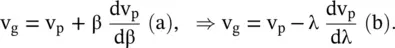

The condition for the normal dispersion is dv p/dβ < 0, dv p/dλ > 0 and for the anomalous dispersion, it is dv p/dβ > 0, dv p/dλ < 0.

The velocity of EM‐wave propagation in a dispersive medium has been discussed in the previous section. The transmission line is a 1D wave‐supporting medium. The lossy line is a dispersive medium, whereas a lossless line, modeled through the line constants L and C, is a nondispersive medium. It acts as a low‐pass filter (LPF). This section shows that a reactively loaded lossless line could be a dispersive medium . A variety of transmission line structures with interesting properties can be developed by using several additional combinations of C and L. Such line structures can be realized with the lumped elements and also by the modification of planar transmission lines. The transmission medium with negative relative permittivity and negative relative permeability has been synthesized with the help of the modified, i.e. reactively loaded line structures. These wave supporting media form a new class of materials known as the metamaterials . They do not exist in nature. However, these novel media have been developed with the defects in the transmission line and using the embedded resonators in the transmission line [B.19, J.8]. The present section considers only an infinitesimal section of the transmission line, modeled as a lumped circuit elements network. The modeled network is reactively loaded to get the loaded line. However, in practice, a finite length of the line is periodically loaded with reactance. Such reactively loaded lines offer novel and improved designs of microwave components and circuits. The periodically loaded line, creating the 1D – EBG and metalines are discussed in the chapters 19and 22.

Figure (3.27a)shows the shunt inductor loaded line structure. An infinitesimally small Δx line length is considered. The cascading of a large number line sections, under the condition Δx → 0, forms a continuous line. The standard Δx long host transmission line section is modeled by the distributed line constants L and C p.u.l. The host line section is loaded with the inclusion , i.e. with additional shunt inductance L sh. The loading element, i.e. inclusion is shown in the gray box, so the periodic embedding of reactive inclusion in the host line medium creates an artificial 1D mixture medium. The concept of the mixture material is further discussed in subsection (6.3.1) of chapter 6.

The inclusion lumped shunt inductance L shdistributed over the length Δx is (L sh/Δx) p.u.l . The total series inductance, (L Δx), gives the total series impedance Z = j ωL Δx and a combination of shunt capacitance (C Δx) and shunt inductance (L sh/Δx) gives the total shunt admittance, Y = j (ωCΔx − Δx/(ωL sh)). The transmission line equations for the shunt inductor loaded line are obtained as follows: