Anand K. Verma - Introduction To Modern Planar Transmission Lines
Здесь есть возможность читать онлайн «Anand K. Verma - Introduction To Modern Planar Transmission Lines» — ознакомительный отрывок электронной книги совершенно бесплатно, а после прочтения отрывка купить полную версию. В некоторых случаях можно слушать аудио, скачать через торрент в формате fb2 и присутствует краткое содержание. Жанр: unrecognised, на английском языке. Описание произведения, (предисловие) а так же отзывы посетителей доступны на портале библиотеки ЛибКат.
- Название:Introduction To Modern Planar Transmission Lines
- Автор:
- Жанр:
- Год:неизвестен
- ISBN:нет данных
- Рейтинг книги:4 / 5. Голосов: 1
-
Избранное:Добавить в избранное
- Отзывы:
-
Ваша оценка:
Introduction To Modern Planar Transmission Lines: краткое содержание, описание и аннотация
Предлагаем к чтению аннотацию, описание, краткое содержание или предисловие (зависит от того, что написал сам автор книги «Introduction To Modern Planar Transmission Lines»). Если вы не нашли необходимую информацию о книге — напишите в комментариях, мы постараемся отыскать её.
rovides a comprehensive discussion of planar transmission lines and their applications, focusing on physical understanding, analytical approach, and circuit models
Planar transmission lines form the core of the modern high-frequency communication, computer, and other related technology. This advanced text gives a complete overview of the technology and acts as a comprehensive tool for radio frequency (RF) engineers that reflects a linear discussion of the subject from fundamentals to more complex arguments.
Introduction to Modern Planar Transmission Lines: Physical, Analytical, and Circuit Models Approach Emphasizes modeling using physical concepts, circuit-models, closed-form expressions, and full derivation of a large number of expressions Explains advanced mathematical treatment, such as the variation method, conformal mapping method, and SDA Connects each section of the text with forward and backward cross-referencing to aid in personalized self-study
is an ideal book for senior undergraduate and graduate students of the subject. It will also appeal to new researchers with the inter-disciplinary background, as well as to engineers and professionals in industries utilizing RF/microwave technologies.
Introduction To Modern Planar Transmission Lines — читать онлайн ознакомительный отрывок
Ниже представлен текст книги, разбитый по страницам. Система сохранения места последней прочитанной страницы, позволяет с удобством читать онлайн бесплатно книгу «Introduction To Modern Planar Transmission Lines», без необходимости каждый раз заново искать на чём Вы остановились. Поставьте закладку, и сможете в любой момент перейти на страницу, на которой закончили чтение.
Интервал:
Закладка:
3.4.2 Circuit Models of Dispersive Transmission Lines
The above discussion demonstrates that the reactive loading of a line modifies the electrical characteristics of an unloaded host line. This section considers a few such modifications.
Shunt Inductor Loaded Line
The total series impedance and total shunt admittance of the shunt inductor loaded dispersive line, shown in Fig (3.27a), are given by
(3.4.12) 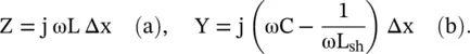
The series impedance and shunt admittance per unit length ( p.u.l .) are
(3.4.13) 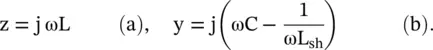
The complex propagation constant of the wave on the shunt inductor loaded line is
(3.4.14) 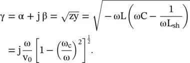
The propagation constant β for ω > ω cis identical to equation (3.4.8). The attenuation constant α is obtained for ω < ω c. The expressions for the phase velocity and group velocity follow from the expression of β as discussed previously. The characteristic impedance of the loaded dispersive transmission line Z od(ω) is given by
(3.4.15) 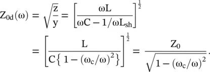
For the case, ω < ω c, the characteristic impedance Z odis an imaginary quantity that stops the signal transmission through the line. The line behaves like a high‐pass filter (HPF). For the case ω > ω c, the characteristic impedance Z odis a real quantity that allows the signal propagation on the line. However, the characteristic impedance Z odin the pass‐band is frequency‐dependent.
Backward Wave Supporting Line
Figure (3.28a)shows the circuit model of the standard low‐pass filter (LPF) type LC transmission line that can also be realized by cascading several lumped elements LC unit cells. However, the distance between two units cells should be a fraction of wavelength, i.e. number of LC unit cells should 10 or more per wavelength. Figure (3.28b)shows the dual of the LC line realized again by cascading several lumped elements CL unit cells. It is called the CL transmission line . It is a high‐pass filter (HPF) type transmission line. Its propagation characteristic is obtained using the circuit analysis:
(3.4.16) 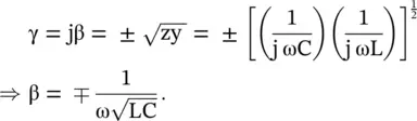
Equation (3.4.16)gives the rectangular hyperbolic relationship for ω and β in the first and second quadrants of the (ω − β) diagram shown in Fig (3.28c). The phase velocity is
(3.4.17) 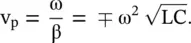
The group velocity is obtained separately for both the negative and positive propagation constants:
(3.4.18) 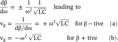
The phase velocity and group velocity are in opposite directions to each other, i.e. v g> 0, v p< 0 or v g< 0, v p> 0. This kind of wave is called the backward wave . If the power is moving from the source to load in the positive direction, the group velocity is in the positive direction from the source to the load, i.e. from the left side to the right side of Fig (3.28b). The power always flows from the source to load. Therefore, the direction of the power flow decides the direction of the EM‐wave propagation . Normally, the direction of the group velocity is in the direction of the power flow. However, the phase velocity appears to be from load to the source . It means at the end of a CL line section the leading phase shift is obtained. It is unlike the lagging phase shift for an LC line section .
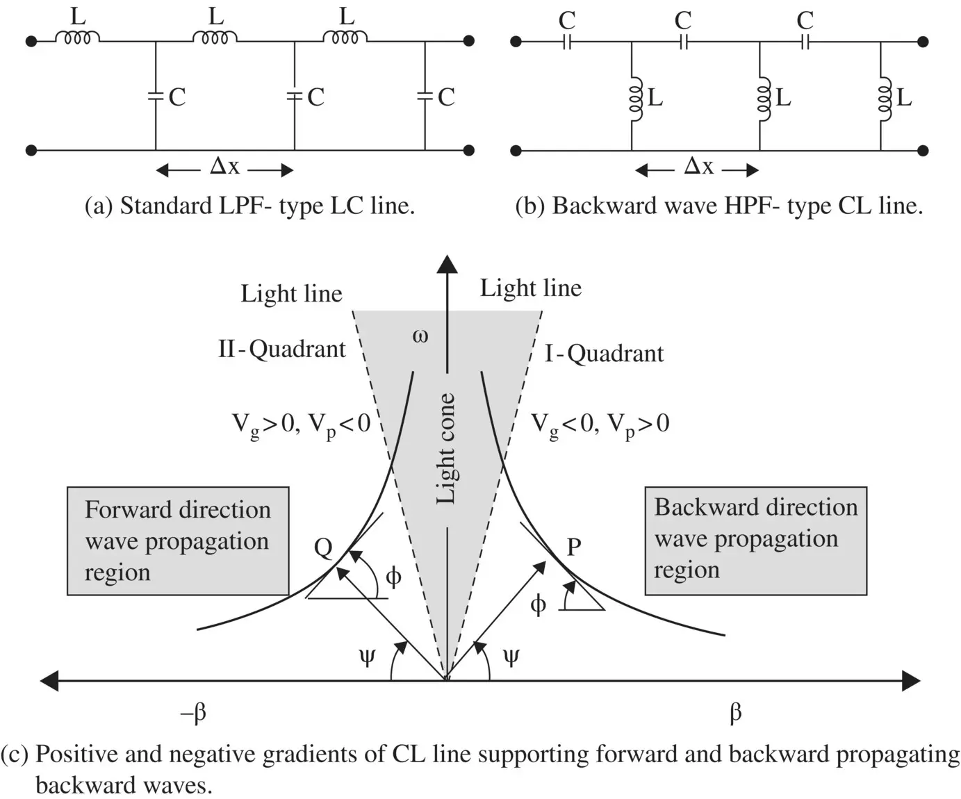
Figure 3.28 Lumped elements models of short transmission line sections and dispersion diagram of CL line.
Figure (3.28c)shows the above results on the (ω − β) diagram. In both the quadrants, the slope ψ at the origin determines the phase velocity, and the local slopes ϕ at the points P and Q determine the group velocities. Both these slopes rapidly increase with an increase in frequency, showing the fast increase in both velocities as given by equations (3.4.17)and (3.4.18). Thus, the lossless CL‐line is a highly dispersive medium . The slope at the origin and the local slope have opposite sense, i.e. one is clockwise and another is anti‐clockwise, showing the antiparallel nature of the phase and group velocities. Such waves are the backward waves . The second quadrant with v g> 0, v p< 0 shows the positive direction of backward wave propagation, while the first quadrant with v g< 0, v p> 0 shows the negative direction of backward wave propagation, i.e. the reflected wave on the CL‐line. The wave in the shaded light‐cone region is fast‐wave, whereas outside the light‐cone it is the slow‐wave.
Equations (3.4.16)and (3.4.17)show that the propagation constant β decreases with an increase in frequency, whereas the phase velocity increases with an increase in frequency. Therefore, the CL‐line has an anomalous dispersion. It is a highly dispersive transmission line. In the case of the material medium, the backward wave with the anomalous dispersion is associated with the strong absorption region. It is discussed in the subsection (6.5.1) of chapter‐6 using the Lorentz model. The standard LPF type transmission line is known as the right hand, i.e. the RH‐transmission line and the HPF type transmission line supporting the backward wave is known as the left hand, i.e. the LH‐transmission line . The RH‐line corresponds to the double‐positive ( DPS ), i.e. both μ, ε positive medium, whereas the LH‐line corresponds to the double negative (DNG ), i.e. both μ, ε negative medium. These media are discussed in section (5.5)of chapter 5. The composite RH‐LH (CRLH)‐transmission line, giving some unique transmission characteristics, models the so‐called metamaterials with negative permittivity and negative permeability [B.19, J.8]. This section considers only one isolated LC unit. The cascading of several such units forms the backward wave supporting LH‐transmission line known as the metalines . It is further discussed in chapter 22.

Figure 3.29 Inductor loaded CL‐line.
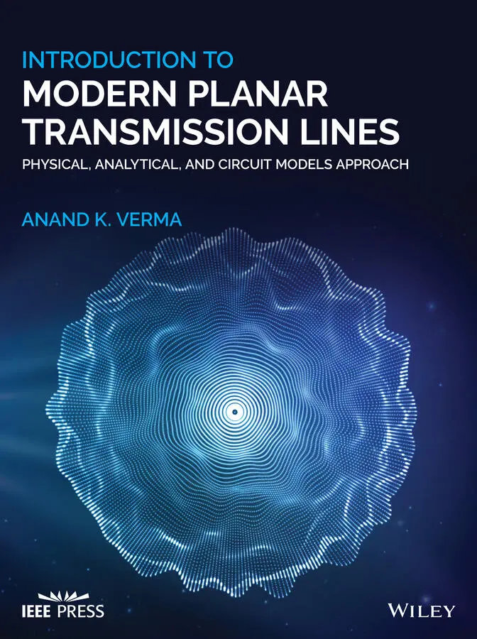
Series Connected Parallel L sh‐C Type Line
The backward wave supporting CL‐line, discussed above, has no cut‐off frequency. Figure (3.29)shows the modified CL‐ line by adding a shunt inductor L sh, inside the gray box, across the series‐connected capacitor C. It is an HPF type CL‐line that supports the backward wave with a cut‐off frequency. The propagation characteristics of this line are obtained from the series impedance and shunt admittance p.u.l .:
Читать дальшеИнтервал:
Закладка:
Похожие книги на «Introduction To Modern Planar Transmission Lines»
Представляем Вашему вниманию похожие книги на «Introduction To Modern Planar Transmission Lines» списком для выбора. Мы отобрали схожую по названию и смыслу литературу в надежде предоставить читателям больше вариантов отыскать новые, интересные, ещё непрочитанные произведения.


Обсуждение, отзывы о книге «Introduction To Modern Planar Transmission Lines» и просто собственные мнения читателей. Оставьте ваши комментарии, напишите, что Вы думаете о произведении, его смысле или главных героях. Укажите что конкретно понравилось, а что нет, и почему Вы так считаете.