Mantle Convection and Surface Expressions

SIsentropic bulk modulus.

*Original data were refit to the finite‐strain formalism of Stixrude & Lithgow‐Bertelloni (2005).

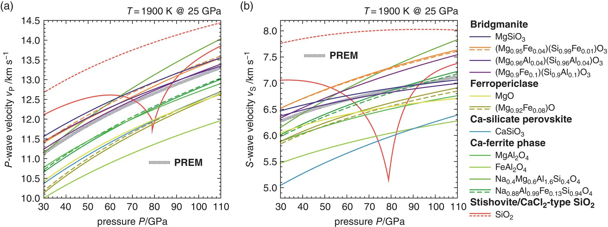
Figure 3.7 P -wave (a) and S -wave (b) velocities for different mineral phases and compositions along a typical adiabatic compression path starting at 1900 K and 25 GPa (see Figure 3.8). These mineral phases and compositions were mixed to model elastic wave speeds of rocks as shown in Figures 3.8and 3.9. Dashed curves show P‐ and S‐ wave velocities when the effect of relevant continuous phase transitions on elastic properties is ignored. See Table 3.1for references.

Chemical bulk compositions for pyrolite and metabasalt were approximated by the depleted MORB mantle (DMM) and NMORB compositions of Workman and Hart (2005). In analogy to the approach of Xu et al. (2008), a hypothetical harzburgite composition was generated by assuming pyrolite to be an 80:20 mixture of harzburgite:basalt by mass. A basalt fraction of 20% in the mantle corresponds to the upper limit of estimates based on geochemical (Morgan & Morgan, 1999; Sobolev et al., 2007) and geodynamical arguments (Ballmer et al., 2015; Nakagawa et al., 2010). For pyrolite and harzburgite, mineral compositions were computed in the system CFMAS and for metabasalt in the system NCFMAS. Bulk compositions were partitioned into the phase assemblages bm‐fp‐cp for pyrolite and harzburgite and bm‐cp‐cf‐st for metabasalt resulting in approximate volume fractions of 77:16:7 (bm:fp:cp) in pyrolite, 74:24:2 (bm:fp:cp) in harzburgite, and 45:26:14:15 (bm:cp:cf:st) in metabasalt, respectively. For each phase, the compositions listed in Table 3.1were mixed to match the computed mineral compositions as outlined in Section 3.6. For some mineral compositions, this approach required extrapolations beyond the compositional limits defined by the mineral compositions in Table 3.1. In these cases, the extrapolations of elastic moduli were restricted to not transcend compositional limits by more than 10% of the compositional range delimited by the mineral compositions of Table 3.1.

The exact mineral compositions and volume fractions for a given bulk rock composition depend critically on assumptions about element partitioning between minerals and the overall Fe 3+/∑Fe ratio. To separate the effects of temperature and compositional parameters, I first computed P‐ and S‐ wave velocities for each bulk rock composition setting Fe 3+/∑Fe = 0.5 in bridgmanite for all rock compositions and requiring that (Fe/Mg) bm/(Fe/Mg) fp= 0.5 and 0.2 in pyrolite and harzburgite, respectively ( Figure 3.6a), and that (Fe/Mg) bm/(Fe/Mg) cf= 1 and (Al/Mg) bm/(Al/Mg) cf= 0.2 in metabasalt ( Figure 3.6b). For these reference scenarios, I computed adiabatic compression paths for each rock composition starting at 1900 K, 1400 K, and 2400 K at 25 GPa and mapped P‐ and S‐ wave velocities between these compression paths based on the Voigt‐Reuss‐Hill average over all relevant mineral phases.

Figure 3.8shows the modeling results for the reference scenario of each bulk rock composition in terms of deviations of the computed P‐ and S‐ wave velocities from the seismic velocities of the preliminary reference Earth model (PREM; Dziewonski & Anderson, 1981):

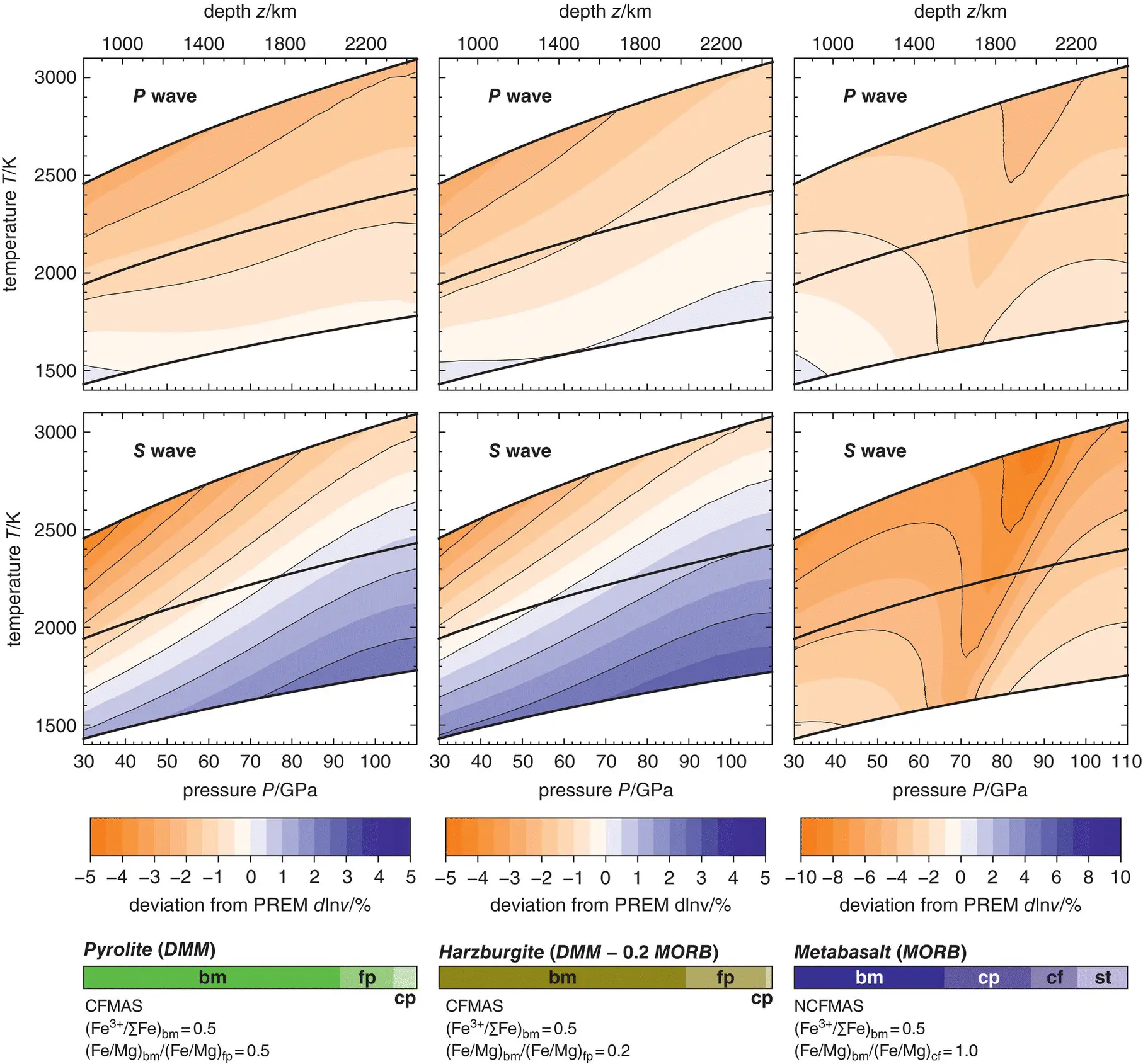
Figure 3.8 Relative contrasts between modeled P -wave (upper row) and S -wave (lower row) velocities for pyrolitic (left column), harzburgitic (central column), and basaltic (right column) bulk rock compositions and PREM. Black curves show adiabatic compression paths for each rock composition and starting at 1400 K, 1900 K, and 2400 K at 25 GPa. For each rock composition, computed volume fractions of minerals and the choice of compositional space and parameters are given below the respective diagrams. See text for details of elastic wave speed modeling.

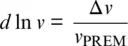
where v PREMstands for the P‐ or S‐ wave velocity of PREM at the respective pressure and Δ v = v − v PREMis the difference in velocity between the model and PREM. P‐ wave velocities of pyrolite appear to systematically fall below those of PREM except for combinations of lowest pressures and temperatures. With magnitudes of less than 3%, these deviations are similar in magnitude to the combined uncertainties on computed P‐ wave velocities that arise from propagating uncertainties on finite‐strain parameters, averaging over elastic anisotropy, and mixing mineral compositions with different elastic properties ( Figures 3.1and 3.3a). While affected by the same sources of uncertainties, computed S‐ wave velocities appear to be more sensitive to temperature than P‐ wave velocities and match S‐ wave velocities of PREM, i.e., d ln v S= 0, within the considered temperature interval. The match with PREM would imply a temperature profile that deviates substantially from any of the computed adiabatic compression paths. Modeled S‐ wave velocities match those of PREM for temperatures below the central adiabat down to a depth of around 1800 km where temperatures would need to rise above those of the central adiabat in order to follow PREM. Projecting the pyrolitic temperature profile for d ln v S= 0 onto the corresponding map for P‐ wave velocities would lead to deviations of –1.5% < d ln v P< 0%. Maps of deviations d ln v for harzburgite are similar to those for pyrolite. However, S‐ wave velocities of harzburgite seem to be systematically higher than those of pyrolite by about 0.5% to 1%, and P‐ wave velocities show slightly steeper gradients with depths. Computed P -wave and in particular S‐ wave velocities for metabasalt are significantly lower than those of PREM at most pressure–temperature combinations explored here. Despite the low volume fraction of free SiO 2phases that go through the phase transition from stishovite to CaCl 2‐type SiO 2, the related elastic softening of the shear modulus gives rise to a pronounced trough of amplified negative contrasts in P‐ and S‐ wave velocities between metabasalt and PREM.

While the maps shown in Figure 3.8illustrate the temperature dependence of P‐ and S‐ wave velocity deviations from PREM, they heavily rely on assumptions about the Fe 3+/∑Fe ratio in bridgmanite and about Fe‐Mg exchange between mineral phases. To explore the impact of these compositional parameters on computed P‐ and S‐ wave velocities, I varied the Fe 3+/∑Fe ratio of bridgmanite and the Fe‐Mg exchange coefficients between bridgmanite and ferropericlase in pyrolite and harzburgite and between bridgmanite and the CF phase in metabasalt within the ranges suggested by data plotted in Figures 3.6a and 3.6b. When varying one compositional parameter, all other parameters were fixed to their values in the references scenarios. Figure 3.9shows the resulting deviations of P‐ and S‐ wave velocities from PREM assuming a range of Fe 3+/∑Fe ratios in bridgmanite or different Fe‐Mg exchange coefficients for each bulk rock composition along the central adiabats shown in Figure 3.8. Computed P‐ and S‐ wave velocities of both pyrolite and harzburgite are more sensitive to changes in the Fe‐Mg exchange coefficient between bridgmanite and ferropericlase than to changes in the Fe 3+/∑Fe ratio of bridgmanite. The sensitivity to Fe‐Mg exchange increases with depth, in particular for S waves. When combined with a reduction of the Fe‐Mg exchange coefficient with depth as suggested by recent computational studies (Muir & Brodholt, 2016; Xu et al., 2017), the strong sensitivity of P‐ and S‐ wave velocities to Fe‐Mg exchange between bridgmanite and ferropericlase could result in substantial velocity reductions for peridotitic rocks towards the lowermost mantle, even along typical adiabatic temperature profiles.