Fabio Giannino - Electromagnetic Methods in Geophysics

Здесь есть возможность читать онлайн «Fabio Giannino - Electromagnetic Methods in Geophysics» — ознакомительный отрывок электронной книги совершенно бесплатно, а после прочтения отрывка купить полную версию. В некоторых случаях можно слушать аудио, скачать через торрент в формате fb2 и присутствует краткое содержание. Жанр: unrecognised, на английском языке. Описание произведения, (предисловие) а так же отзывы посетителей доступны на портале библиотеки ЛибКат.

Electromagnetic Methods in Geophysics: краткое содержание, описание и аннотация

Предлагаем к чтению аннотацию, описание, краткое содержание или предисловие (зависит от того, что написал сам автор книги «Electromagnetic Methods in Geophysics»). Если вы не нашли необходимую информацию о книге — напишите в комментариях, мы постараемся отыскать её.

Discover the utility of four popular electromagnetic geophysical techniques In
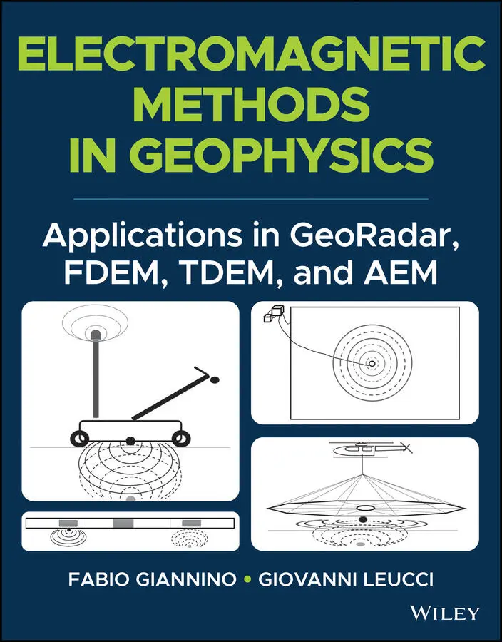
, accomplished researchers Fabio Giannino and Giovanni Leucci deliver an in-depth exploration of the theory and application of four different electromagnetic geophysical techniques: ground penetrating radar, the frequency domain electromagnetic method, the time domain electromagnetic method, and the airborne electromagnetic method. The authors offer a full description of each technique as they relate to the economics, planning, and logistics of deploying each of them on-site.
The book also discusses the potential output of each method and how it can be combined with other sources of below- and above-ground information to create a digitized common point cloud containing a wide variety of data.
Giannino and Leucci rely on 25 years of professional experience in over 40 countries around the world to provide readers with a fulsome description of the optimal use of GPR, FDEM, TDEM, and AEM, demonstrating their flexibility and applicability to a wide variety of use cases.
Readers will also benefit from the inclusion of:
A thorough introduction to electromagnetic theory, including the operative principles and theory of ground penetrating radar (GPR) and the frequency domain electromagnetic method (FDEM) An exploration of hardware architecture and surveying, including GPR, FDEM, time domain electromagnetic method (TDEM), and airborne electromagnetic (AEM) surveying A collection of case studies, including a multiple-geophysical archaeological GPR survey in Turkey and a UXO search in a building area in Italy using FDEM /li> Discussions of planning and mobilizing a campaign, the shipment and clearance of survey equipment, and managing the operative aspects of field activity Perfect for forensic and archaeological geophysicists,
will also earn a place in the libraries of anyone seeking a one-stop reference for the planning and deployment of GDR, FDEM, TDEM, and AEM surveying techniques.

Electromagnetic Methods in Geophysics — читать онлайн ознакомительный отрывок

Ниже представлен текст книги, разбитый по страницам. Система сохранения места последней прочитанной страницы, позволяет с удобством читать онлайн бесплатно книгу «Electromagnetic Methods in Geophysics», без необходимости каждый раз заново искать на чём Вы остановились. Поставьте закладку, и сможете в любой момент перейти на страницу, на которой закончили чтение.

Тёмная тема
Сбросить

Интервал:

Закладка:

Сделать
Figure 7.50 Area 2: the 3D representation by iso‐surface amplitude of the EM...Figure 7.51 Area 2: excavation results.Figure 7.52 Area 3: the processed radar sections.Figure 7.53 Area 3: excavation results.Figure 7.54 Location of the Crypt of the ‘Spirito Santo’ in Monopoli.Figure 7.55 Fresco inside the crypt.Figure 7.56 The surveyed wall.Figure 7.57 The frequency slices.Figure 7.58 Comparison between (a) the frequency slice in the interval 700–7...Figure 7.59 Comparison between (a) photo; (b) the distribution of temperatur...Figure 7.60 Area T01 at the abutment of the tunnel.Figure 7.61 Area T02 at the ceiling of the tunnel.Figure 7.62 An image of the C thrue GPR while collecting data at Area T01.Figure 7.63 An image of the TR900 antenna while collecting data at Area T01....Figure 7.64 result of the C thrue at T01.Figure 7.65 result of the TR900 at T01.Figure 7.66 result of the C thrue at T02.Figure 7.67 Volumetric water content (w) as function of relative dielectric ...Figure 7.68 Cubic concrete sample used for test measurement.Figure 7.69 (a) GPR Traveltime Tomography scheme, (b) ray tracing, (c) first...Figure 7.70 GPR Travel‐time Tomography relative dielectric constant (k) and ...Figure 7.71 co‐pole configuration: (a) co‐polarized, (b) cross‐polarized.Figure 7.72 reinforced bar orientation: (a) parallel to the long axis of a d...Figure 7.73 (a) The resulting hyperbola from cylindrical object; (b) general...Figure 7.74 (a) synthetic model with a metal bar of 10mm diameter, (b) synth...Figure 7.75 Real GPR data acquired on a bar with diameter of 20mm.Figure 7.76 synthetic model with metal bars of 8 to 10mm diameters.Figure 7.77 synthetic radar sections: (a) bar signals along the EM field, (b...Figure 7.78 The synthetic radar time section processed.Figure 7.79 The controlled test scheme.Figure 7.80 The GPR processed data: (a) normal polarization, (b) parallel po...Figure 7.81 bar diameters versus Ac/An ratio obtained using both the forward...Figure 7.82 Test data on known bar diameters of 20mm: (a) normal polarizatio...Figure 7.83 Test data on known bar diameters of 6mm: (a) normal polarization...Figure 7.84 The Basilica di Santa Croce.Figure 7.85 Phase of the GPR data acquisition. On the right side of the phot...Figure 7.86 location of GPR profiles.Figure 7.87 the processed radar sections.Figure 7.88 Time slices 18‐27cm: (a) left side, (b) central side, (c) right ...Figure 7.89 the iso‐surface.Figure 7.90 Photos of the excavation done after the results of geophysics.Figure 7.91 the survey area in Italy.Figure 7.92 The survey area and its dimension.Figure 7.93 The Stream UP system.Figure 7.94 Coverage of the GPR survey. Blue polygons indicate the footprint...Figure 7.95 Tomography view at 60cm below ground. Black arrows point at the ...Figure 7.96 Tomography view at 71cm below ground. Black arrows point at the ...Figure 7.97 Tomography view at 75cm below ground. Black arrows point at the ...Figure 7.98 Tomography view at 90cm below ground. Black arrows point at the ...Figure 7.99 Tomography view at 101cm below ground. Black arrows point at the...Figure 7.100 Tomography view at 110cm below ground. Black arrows point at th...Figure 7.101 Tomography view at 60cm below ground. The green solid lines are...Figure 7.102 tomography view at 76cm below ground. The green solid lines are...Figure 7.103 Tomography view at 90cm below ground. The green solid lines are...Figure 7.104 export of the targets in CAD compatible format.Figure 7.105 the survey area in Scandinavia.Figure 7.106 The survey area and its dimension.Figure 7.107 The Stream C system during the site operations.Figure 7.108 Coverage of the GPR survey. Blue polygons indicate the footprin...Figure 7.109 tomography view at 43cm below ground.Figure 7.110 tomography view at 59 cm below ground.Figure 7.111 tomography view at 61 cm below ground.Figure 7.112 tomography view at 65 cm below ground.Figure 7.113 tomography view at 175 cm below ground.Figure 7.114 Tomography view at 171 cm below ground. The black, red, and yel...Figure 7.115 View of the targets identified. The black, red, and yellow soli...Figure 7.116 Taiwan.Figure 7.117 The Stream EM system.Figure 7.118 The survey area.Figure 7.119 Coverage of the GPR survey at the Taiwan urban site. Blue polyg...Figure 7.120 3D view from top.Figure 7.121 3D view from bottom.Figure 7.122 targets (man‐hole covers in blue, pipes in green, and cavity lo...Figure 7.123 export of the targets from GPR merged with the point cloud of t...Figure 7.124 export of the targets from GPR merged with the point cloud of t...Figure 7.125 export of the targets from GPR merged with the point cloud of t...Figure 7.126 (a) Schematic of the set up for EC1. (b) Picture of the setup....Figure 7.127 Experimental configuration of the setup for two of the experime...Figure 7.128 Layout for the EC3: (a) The SE (metallic wire) on the road surf...Figure 7.129 Radar sections for EC1. From top to bottom: dry condition; slig...Figure 7.130 Radar sections acquired through the 200 MHz antenna. Upper pane...Figure 7.131 Radar sections acquired through the 600 MHz antenna: upper pane...Figure 7.132 Percentage variation of the velocity in the subsoil.Figure 7.133 Georadar profile, perpendicular to the pipe, acquired through t...Figure 7.134 Upper panel: B‐scan with the antenna at 600 MHz; lower panel: B...Figure 7.135 Zoom on the Bscan of fig. 15 upper panel.Figure 7.136 Orthogonal profiles at the abscissas 16.4 m and 18 m.Figure 7.137 Location of the survey site: via Luca Antonio Resta, Mesagne, (...Figure 7.138 South‐West Brindisi Provincia Geological Map;Figure 7.139 Photos: a) example of cracks (labeled L) developed in several b...Figure 7.140 Comparison between data set (500 MHz antenna) before (a) and af...Figure 7.141 Time slice for the 20–34 ns time window (0.7 m–1.2 m depth). T ...Figure 7.142 (a) (top) Raw radar section. Velocity analysis with the diffrac...Figure 7.143 Lateral velocity variations across the area in the time window ...Figure 7.144 The IDS GeoRadar HiBrigHT GPR System.Figure 7.145 The survey acquisition scheme.Figure 7.146 The survey acquisition scheme.Figure 7.147 data acquisition lines marked on asphalt with chalk (indicated ...Figure 7.148 The Tomography view of the migrated data (amplitude of the EM s...Figure 7.149 the export of the points of reflection of the GPR signal due to...Figure 7.150 The B scans at Area 1.Figure 7.151 The B scans at Area 1.Figure 7.152 The Amplitude Map at Area 1.Figure 7.153 The Moisture Map at Area 1.Figure 7.154 The Concrete Map at Area 1.Figure 7.155 Survey area. Red polygon indicates the area where FDEM measurem...Figure 7.156 Survey area. The red polygon indicates the area where FDEM meas...Figure 7.157 The data acquisition phase with the Geonics EM 31.Figure 7.158 FDEM results. Apparent Conductivity map relating with the acqui...Figure 7.159 FDEM results. In Phase component map relating with the acquisit...Figure 7.160 Survey area. Red polygon indicates the area where FDEM measurem...Figure 7.161 Survey area. Red polygon indicates the area where FDEM measurem...Figure 7.162 Survey area. Preparation of the trial field. Placing the bricks...Figure 7.163 Survey area. Preparation of the trial field. Placing the tires ...Figure 7.164 Survey area. Preparation of the trial field. Placing the metal ...Figure 7.165 Survey area. GPS positions of the acquisition lines.Figure 7.166 FDEM results with GSSI EMP‐400 Profiler. Apparent Electrical Co...Figure 7.167 FDEM results with GSSI EMP‐400 Profiler. Apparent Electrical Co...Figure 7.168 FDEM results with GSSI EMP‐400 Profiler. Apparent Electrical Co...Figure 7.169 FDEM results with GSSI EMP‐400 Profiler. In phase component map...Figure 7.170 FDEM results with GSSI EMP‐400 Profiler. In phase component map...Figure 7.171 FDEM results with GSSI EMP‐400 Profiler. In phase component map...Figure 7.172 FDEM results with GSSI EMP‐400 Profiler. Quadrature component m...Figure 7.173 FDEM results with GSSI EMP‐400 Profiler. Quadrature component m...Figure 7.174 FDEM results with GSSI EMP‐400 Profiler. Quadrature component m...Figure 7.175 FDEM results with Geonics EM31. Apparent Electrical Conductivit...Figure 7.176 FDEM results with Geonics EM31. Apparent Electrical Conductivit...Figure 7.177 FDEM results with GSSI EMP‐400 Profiler. Apparent Electrical Co...Figure 7.178 Survey area. Red polygon indicates the area where FDEM measurem...Figure 7.179 Survey area. Red polygon indicates the area where FDEM measurem...Figure 7.180 Survey area. Sub‐area 1. Blue lines indicate the GPS positions ...Figure 7.181 Survey area. Sub‐area 2. Blue lines indicate the GPS positions ...Figure 7.182 Survey area. Sub‐area 4. Blue lines indicate the GPS positions ...Figure 7.183 Survey area. Sub‐area 5. Blue lines indicate the GPS positions ...Figure 7.184 FDEM results with GSSI EMP‐400 Profiler. Apparent electrical Co...Figure 7.185 FDEM results with GSSI EMP‐400 Profiler. Apparent electrical Co...Figure 7.186 FDEM results with GSSI EMP‐400 Profiler. Apparent electrical Co...Figure 7.187 Image of the survey area with indication of a few elements usef...Figure 7.188 Apparent Electrical Conductivity map at 2 KHz, superimposed to ...Figure 7.189 Apparent Electrical Conductivity map at 9 KHz, superimposed to ...Figure 7.190 Apparent Electrical Conductivity map at 15 KHz, superimposed to...Figure 7.191 Aerial photo of the survey area. Here the points named A, B, C ...Figure 7.192 Survey area. The yellow circle indicates the presence of two ho...Figure 7.193 Apparent Conductivity map.Figure 7.194 In Phase Component map.Figure 7.195 Apparent Electric Conductivity map overlaid to aerial photo.Figure 7.196 In Phase Component map overlaid to aerial photo.Figure 7.197 Location map of the Italian reference and calibration site. (a)...Figure 7.198 The Geonics 47 data calibrated at the Lyngby test site (Denmark...Figure 7.199 Signal and noise responses measured for the ultra‐high (UH), ve...Figure 7.200 WSW–ENE resistivity section. Smooth inversion results calculate...Figure 7.201 Field data (error bar), forward responses (solid line) and reco...Figure 7.202 Joint inversion result of the collected Geonics 47 and WalkTEM ...Figure 7.203 (a) 1‐D reference resistivity model of the San Rossore referenc...Figure 7.204 Comparison between the reference response (blue curve) and the ...Figure 7.205 (a) Forward response of the calibrated 100 × 100 m loop data pl...Figure 7.206 Location and digital elevation model of the Spiritwood AeroTEM ...Figure 7.207 Inversion results for the AeroTEM survey. The recovered 1D resi...Figure 7.208 (a) AeroTEM and (b) VTEM resistivity models along seismic line ...Figure 7.209 Histogram of layer resistivities for all 1D 29‐layer smooth inv...Figure 7.210 Automatic segmentation of lithology for model cross section M1 ...Figure 7.211 AeroTEM resistivity along model cross section M2. Solid black l...Figure 7.212 Ground‐based TEM data and inversion results forc80 × 80 m centr...Figure 7.213 AeroTEM resistivity along model cross section M3. The solid bla...Figure 7.214 A 3D depiction of the bottom erosional surfaces of all buried v...Figure 7.215 Bedrock topography of the 3D geologic model obtained via interp...Figure 7.216 (a) Seismic reflection profiles S2 (left) and S6 (right). Red l...Figure 7.217 (a) Three‐dimensional voxel‐based lithological model of a selec...Figure 7.218 (a) VTEM resistivity model along seismic line S1. (b) A 3D depi...Figure 7.219 The 3D visualization of the voxel‐based geologic model of the b...Figure 7.220 EM survey lines over government geological map. For comparison ...Figure 7.221 Example of transients affected by IP (red bars represent negati...Figure 7.222 Distribution of sum of log10(abs(∑(negatives)), in pV/Am4 (abov...Figure 7.223 Distribution of time constant τ over interval C (cf Table 7.2)....Figure 7.224 Scatter plot and corresponding linear regression showing correl...Figure 7.225 Sensitivity of IP scanner to the metric of decay rate interval ...Figure 7.226 Sensitivity of IP scanner to the metric of decay rate interval ...Figure 7.227 Sensitivity of IP scanner to the metric of the sum of negatives...Figure 7.228 “AIP scanner” map, with dark blue = no AIP, yellow‐orange‐red =...Figure 7.229 Inverted chargeability section compared against profile of AIP ...Figure 7.230 Resistivity models obtained with AIP modelling (top) and withou...Figure 7.231 Resistivity models obtained with AIP modelling (top) and withou...Figure 7.232 Chargeability section accompanying Figure 7.231. The fault is e...Читать дальше
Тёмная тема
Сбросить

Интервал:

Закладка:

Сделать

Похожие книги на «Electromagnetic Methods in Geophysics»

Представляем Вашему вниманию похожие книги на «Electromagnetic Methods in Geophysics» списком для выбора. Мы отобрали схожую по названию и смыслу литературу в надежде предоставить читателям больше вариантов отыскать новые, интересные, ещё непрочитанные произведения.


Отзывы о книге «Electromagnetic Methods in Geophysics»

Обсуждение, отзывы о книге «Electromagnetic Methods in Geophysics» и просто собственные мнения читателей. Оставьте ваши комментарии, напишите, что Вы думаете о произведении, его смысле или главных героях. Укажите что конкретно понравилось, а что нет, и почему Вы так считаете.

x