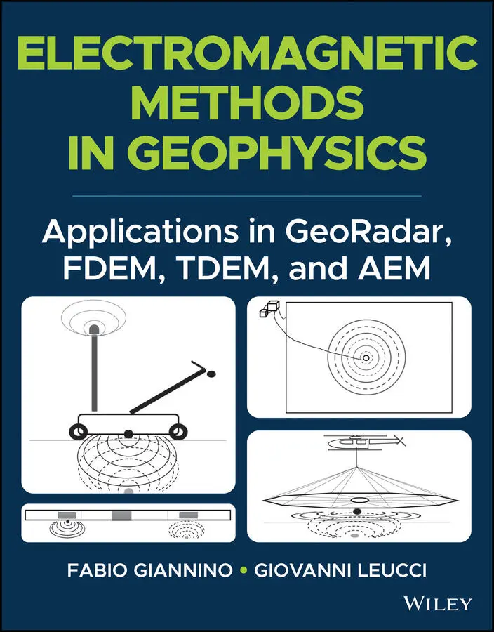
Fabio Giannino - Electromagnetic Methods in Geophysics

3 Chapter 4Figure 4.1 Sketch of an electromagnetometer. Tx is the transmitting coil, Rx...Figure 4.2 GCM Geonics Ltd EM31 MK‐2 during the acquisition phases of a surv...Figure 4.3 GCM GSSI Inc EMP‐400 during the acquisition phases of a survey.Figure 4.4 GCM Dualem 6s, during the acquisition phases of a survey.Figure 4.5 Data acquisition. Possible problems of under‐sampling or over‐sam...Figure 4.6 Data acquisition. Black line represents the possible position of ...Figure 4.7 Data acquisition in the case of an unknown shaped target. In “A” ...Figure 4.8 Data acquisition. In the area bordered by the blue polygon, an in...Figure 4.9 Data acquisition. Stationary acquisition mode (or “Point by Point...Figure 4.10 Data acquisition. Positioning of the stations in the stationary ...Figure 4.11 Data acquisition. Acquisition mode continuous without GNSS.Figure 4.12 Data acquisition. Acquisition mode continuous with GPS.Figure 4.13 Data acquisition. Example of correction of GNSS positions.Figure 4.14 Data acquisition. Example of data shown on the screen of the int...Figure 4.15 Data analysis. Example of GNSS (positioning, geographic coordina...Figure 4.16 Data analysis. Example of data file ready for the following proc...Figure 4.17 Data analysis. Example of Apparent Electric Conductivity map.Figure 4.18 example of the graph showing the in‐phase component with respect...Figure 4.19 example of inverted 2D section of conductivity obtained by using...Figure 4.20 example of inverted 3D map at a given depth of conductivity obta...

4 Chapter 5Figure 5.1 Sketch of the essential (minimum) parts describing a system to ca...Figure 5.2 Scheme of functioning of a TDEM survey.Figure 5.3 1D TDEM sounding.Figure 5.4 Example of 1D model of the subsoil after 1D inversion of TDEM dat...Figure 5.5 Example of 2D section along the XZ plan, obtained after interpola...Figure 5.6 Example of 2D section along the XY plan, obtained after interpola...

5 Chapter 6Figure 6.1 Sketch of the essential (minimum) parts describing a system to ca...Figure 6.2 Scheme of functioning of an AEM survey.Figure 6.3 Typical 1D AEM sounding.Figure 6.4 Example of part of a flight plan for a AEM campaign.Figure 6.5 A data processing window showing portions of data deleted because...Figure 6.6 The trapezoid shaped averaging core: data are averaged over large...Figure 6.7 Altimetry data processing. (a) Raw data, (b) after a first phase ...Figure 6.8 Tilt‐meter data processingFigure 6.9 Data processing. The phase of couplings removal and filtering. Gr...Figure 6.10 Inversion of AEM data. In (d) the actual geological section is i...Figure 6.11 Example of 1D model of the subsoil after 1D inversion of TDEM da...Figure 6.12 Example of Electrical Resistivity 2D section along the XZ plan, ...Figure 6.13 Example of Electrical Resistivity 2D plan along the XY plan, at ...Figure 6.14 Example of Electrical Chargeability 2D plan along the XY plan, a...

6 Chapter 7Figure 7.1 The Martyrium of St Philip planimetry with the surveyed area high...Figure 7.2 The processed radar sections related to the profiles a) 11, b) 19...Figure 7.3 The time slices.Figure 7.4 Iso‐surface visualization of the envelope of the migrated data (5...Figure 7.5 FDEM slice map of the electrical conductivity (EC): a) 14025Hz; b...Figure 7.6 The geophysical surveyed areas.Figure 7.7 Area 2 time slices related to 600MHz antenna GPR data.Figure 7.8 Area 2 time slices related to 200MHz antenna GPR data.Figure 7.9 Area 2: time slices: (a) 75–115 cm depth related to the GPR data ...Figure 7.10 Area 3 time slices related to 600MHz antenna GPR data.Figure 7.11 Area 3 time slices related to 200MHz antenna GPR data.Figure 7.12 Area 3: time slices 290‐320cm depth related to the GPR data acqu...Figure 7.13 Area 3: Examples of three‐dimensional visualizations by means of...Figure 7.14 GPR profiles location: a) on the Sanctuary and its north‐west si...Figure 7.15 Processed radar sections related to the R1, R2 and R3 profile ac...Figure 7.16 Sanctuary: (a) R3 processed radar section, (b) seismic depth sli...Figure 7.17 The Sanctuary GPR depth slices.Figure 7.18 The Sanctuary planimetry overlap the GPR slice at depth ranging ...Figure 7.19 The depth slices at north‐east side of the sanctuary area.Figure 7.20 time slices.Figure 7.21 The Archaeological site of Pyrgi near Santa Severe, Rome (Italy)...Figure 7.22 The Stream X system at Pyrgi site. The excavated sector is in th...Figure 7.23 The survey area.Figure 7.24 Coverage of the GPR survey at the Pyrgi site. Blue polygons indi...Figure 7.25 Time slice at ‐0.2 meters.Figure 7.26 Time slice at ‐0.4 meters.Figure 7.27 Time slice at ‐0.8 meters.Figure 7.28 Time slice at ‐1 meter.Figure 7.29 Lecce ‐ Piazza Duomo. Location of the religious building investi...Figure 7.30 Plan of the Lecce Cathedral. Hypothetical reconstruction of the ...Figure 7.31 Photos (on the left) and plan (on the right) of the crypt under ...Figure 7.32 Lecce Cathedral, crypt under the transept: elaborated radar sect...Figure 7.33 Lecce Cathedral, crypt under the transept: GPR time slice 270 MH...Figure 7.34 Lecce Cathedral, crypt under the transept, GPR time slices (270 ...Figure 7.35 3D iso‐surfaces related to three depth range: (a) 0.0‐1.0 m, (b)...Figure 7.36 Lecce Cathedral: GPR profiles along the northern nave (600 MHz a...Figure 7.37 Lecce Cathedral: GPR profiles along the northern nave (200 MHz a...Figure 7.38 Lecce Cathedral: GPR time slice (200 MHz antenna; depth correspo...Figure 7.39 Lecce Cathedral: GPR time slice (200 MHz antenna; depth correspo...Figure 7.40 Lecce Cathedral: GPR time slice (200 MHz antenna; depth correspo...Figure 7.41 Lecce Cathedral: 3D visualization shows the distribution of the ...Figure 7.42 The study area in Ventarron (north Peru).Figure 7.43 The surveyed areas.Figure 7.44 Area 1: the processed radar section related to profile R5.Figure 7.45 Area 1: Depth slices.Figure 7.46 Area 1: the 3D representation by iso‐surface amplitude of the EM...Figure 7.47 Area 1: exavation results.Figure 7.48 Area 2: the processed radar section related to profile R3.Figure 7.49 Area 2: Depth slices.