Saeid Sanei - EEG Signal Processing and Machine Learning

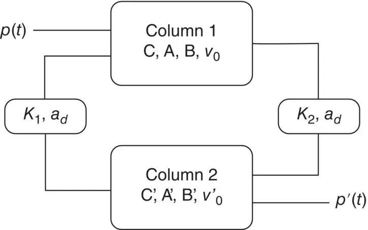
Figure 3.11 A two‐column model for generation of VEP. Two connectivity constants K 1and K 2attenuate the output of a column before it is fed to the other.

These models are basically the description of single and multichannel signals in terms of a limited number of statistical parameters which not only represent the morphology of the waveforms but also their temporal or spatial sample correlations. In these models the internal and external noise is often considered as an uncorrelated temporal signal independent of the brain generated signals.

The main objective of using prediction methods is to find a set of model parameters which best describe the signal generation system. Such models generally require a noise type input. In autoregressive (AR) modelling of signals each sample of a single channel EEG measurement is defined to be linearly related with respect to a number of its previous samples, i.e.:

(3.40)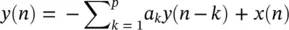

where a k, k = 1,2,…, p , are the linear parameters, n denotes the discrete sample time normalized to unity, p is called the model or prediction order and x ( n ) is the noise input. In an autoregressive moving average (ARMA) linear predictive model each sample is obtained based on a number of its previous input and output sample values, i.e.:

(3.41)

where b k , k = 1, 2,…, q are the additional linear parameters. The parameters p and q are the model orders. The Akaike criterion can be used to determine the order of the appropriate model of a measurement signal by maximizing the log-likelihood equation [22] with respect to the model order:

(3.42)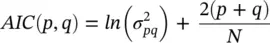

where p and q represent respectively, the assumed AR and MA model prediction orders, N is the number of signal samples, and is the noise power of the ARMA model at the p th and q th stage. Later in this chapter we will see how the model parameters are estimated either directly or by employing some iterative optimization techniques.

In a multivariate AR (MVAR) approach a multichannel scheme is considered. Therefore, each signal sample is defined versus both its previous samples and the previous samples of the signals from other channels, i.e. for channel i we have:

(3.43)

where m represents the number of channels and x i( n ) represents the noise input to channel i . Similarly, the model parameters can be calculated iteratively in order to minimize the error between the actual and predicted values [23].

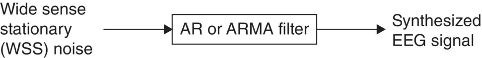
Figure 3.12 A linear model for the generation of EEG signals.

There are numerous applications for linear models. These applications are discussed in other chapters of this book. Different algorithms have been developed to find efficiently the model coefficients. In the maximum likelihood estimation (MLE) method [23–25] the likelihood function is maximized over the system parameters formulated from the assumed real, Gaussian distributed, and sufficiently long input signals of approximately 10–20 seconds (consider a sampling frequency of f s= 250 Hz as often used for EEG recordings). Using Akaike's method the gradient of the squared error is minimized using the Newton–Raphson approach applied to the resultant nonlinear equations [23, 26]. This is considered as an approximation to the MLE approach. In the Durbin method [27] the Yule–Walker equations, which relate the model coefficients to the autocorrelation of the signals, are iteratively solved. The approach and the results are equivalent to those using a least‐squared‐based scheme [28]. The MVAR coefficients are often calculated using the Levinson–Wiggins–Robinson (LWR) algorithm [29]. The MVAR model and its application in representation of what is called a direct transfer function (DTF), and its use in quantification of signal propagation within the brain, will be explained in detail in Chapter 8of this book. After the parameters are estimated the synthesis filter can be excited with wide sense stationary noise to generate the EEG signal samples. Figure 3.12illustrates the simplified system.

The prediction models can be easily extended to multichannel data. This leads to estimation of matrices of prediction coefficients. These parameters stem from both the temporal and interchannel correlations.

Prony's method has been previously used to model EPs [30, 31]. Based on this model an EP, which is obtained by applying a short audio or visual brain stimulus to the brain, can be considered as the impulse response (IR) of a linear infinite impulse response (IIR) system. The original attempt in this area was to fit an exponentially damped sinusoidal model to the data [32]. This method was later modified to model sinusoidal signals [33]. Prony's method is used to calculate the LP parameters. The angles of the poles in the z‐plane of the constructed LP filter are then referred to the frequencies of the damped sinusoids of the exponential terms used for modelling the data. Consequently, both the amplitude of the exponentials and the initial phase can be obtained following the methods used for an AR model, as follows.

Based on the original method we can consider the output of an AR system with zero excitation to be related to its IR as:

(3.44)

where y ( n ) represents the exponential data samples, p is the prediction order, , r k= exp (( α k+ j 2 πf k) T s), T sis the sampling period normalized to 1, A kis the amplitude of the exponential, α kis the damping factor, f kis the discrete‐time sinusoidal frequency in samples per second, and θ jis the initial phase in radians.

Therefore, the model coefficients are first calculated using one of the methods previously mentioned in this section, i.e. , where: