Saeid Sanei - EEG Signal Processing and Machine Learning

(3.30)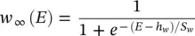

(3.31)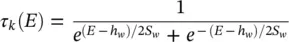

The steady‐state activation function a ca( E ), involved in calculation of the calcium current, is defined as:

(3.32)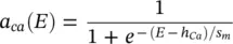

Similar to the sodium current in the Hodgkin–Huxley model, the calcium current is an inward current. Since the calcium activation current is a fast process in comparison with the potassium current, it is modelled as an instantaneous function. This means that for each voltage E , the steady‐state function a Ca( E ) is calculated. The calcium current does not incorporate any inactivation process. The activation variable w khere is similar to a kin the Hodgkin–Huxley model, and finally the leak currents for both models are the same [12]. A simulation of the Morris–Lecar model is presented in Figure 3.6.

Calcium‐dependent potassium channels are activated by intracellular calcium, the higher the calcium concentration the higher the channel activation [12]. For the Morris–Lecar model to exhibit bursting behaviour, the two parameters of maximal time constant and the input current have to be changed [12]. Figure 3.7shows the bursting behaviour of the Morris–Lecar model. The basic characteristics of a bursting neuron are the duration of the spiky activity, the frequency of the APs during a burst, and the duration of the quiescence period. The period of an entire bursting event is the sum of both active and quiescence duration [12].

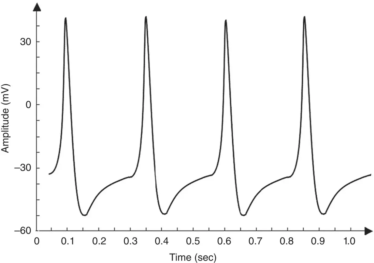
Figure 3.6 Simulation of an AP within the Morris–Lecar model. The model parameters are: C m= 22 μF cm −2, =3.8 mS cm −2, =8.0 mS cm −2, =1.6 mS cm −2, E Ca= 125 mV, E k= −80 mV, E l= −60 mV, λ t= 0.06, h Ca= −1.2, S m= 8.8.

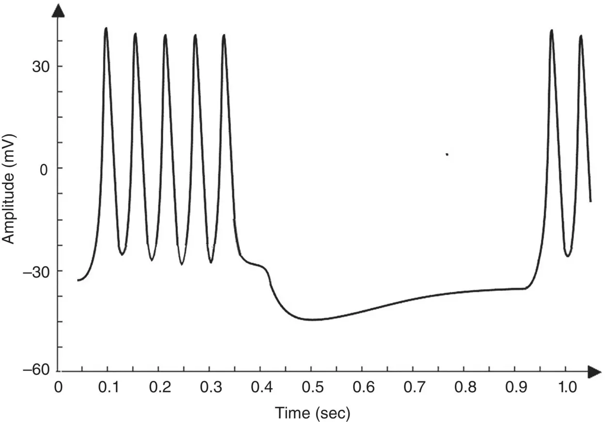
Figure 3.7 An illustration of the bursting behaviour that can be generated by the Morris–Lecar model.

Neurons communicate with each other across synapses through axon‐dendrites or dendrites‐dendrites connections, which can be excitatory, inhibitory, or electric [12]. By combining a number of the above models, a neuronal network can be constructed. The network exhibits oscillatory behaviour due to the synaptic connection between the neurons. It is commonly assumed that excitatory synaptic coupling tends to synchronize neural firing, while inhibitory coupling pushes neurons towards anti‐synchrony. Such behaviour has been seen in models of neuronal circuits [1].

A synaptic current is produced as soon as a neuron fires an AP. This current stimulates the connected neuron and may be modelled by an alpha function multiplied by a maximal conductance and a driving force as:

(3.33)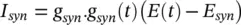

where:

(3.34)

and t is the latency or time since the trigger of the synaptic current, u is the time to reach to the peak amplitude, E synis the synaptic reversal potential, and is the maximal synaptic conductance. The parameter u alters the duration of the current while changes the strength of the current. This concludes the treatment of the modelling of APs.

As the nature of the EEG sources cannot be determined from the electrode signals directly, many researchers have tried to model these processes on the basis of information extracted using signal processing techniques. The method of linear prediction (LP) described in the later sections of this chapter is frequently used to extract a parametric description.

A tutorial on realistic neural modelling using the Hodgkin–Huxley excitation model by David Beeman has been documented at the first annual meeting of the World Association of Modelers (WAM) Biologically Accurate Modeling Meeting (BAMM) in 2005 in Texas, USA. This can be viewed at http://www.brains‐minds‐media.org/archive/218.

The objective in this section is to introduce some established models for generating normal and some abnormal EEGs. These models are generally nonlinear and some have been proposed [15] for modelling a normal EEG signal and some others for the abnormal EEGs.

A simple distributed model consisting of a set of simulated neurons, thalamocortical relay cells, and interneurons was proposed [16, 17] that incorporates the limited physiological and histological data available at that time. The basic assumptions were sufficient to explain the generation of the alpha rhythm, i.e. the EEGs within the frequency range of 8–13 Hz.

A general nonlinear lumped model may take the form shown in Figure 3.8. Although the model is analogue in nature all the blocks are implemented in discrete form. This model can take into account the major characteristics of a distributed model and it is easy to investigate the result of changing the range of excitatory and inhibitory influences of thalamocortical relay cells and interneurons.

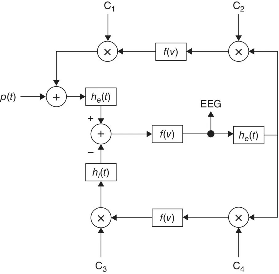
Figure 3.8 A nonlinear lumped model for generating the rhythmic activity of the EEG signals; h e( t ) and h i( t ) are the excitatory and inhibitory post synaptic potentials, f ( v ) is normally a simplified nonlinear function, and the C is are respectively the interaction parameters representing the interneurons and thalamocortical neurons [16].

In this model [16] there is a feedback loop including the inhibitory post‐synaptic potentials, the nonlinear function, and the interaction parameters C 3and C 4. The other feedback includes mainly the excitatory potentials, nonlinear function, and the interaction parameters C 1and C 2. The role of the excitatory neurons is to excite one or two inhibitory neurons. The latter, in turn, serve to inhibit a collection of excitatory neurons. Thus, the neural circuit forms a feedback system. The input p ( t ) is considered as a white noise signal. This is a general model; more assumptions are often needed to enable generation of the EEGs for the abnormal cases. Therefore, the function f ( v ) may change to generate the EEG signals for different brain abnormalities. Accordingly, the C icoefficients can be varied. In addition, the output is subject to environment and measurement noise. In some models, such as the local EEG model (LEM) [16] the noise has been considered as an additive component in the output.