Saeid Sanei - EEG Signal Processing and Machine Learning

(3.45)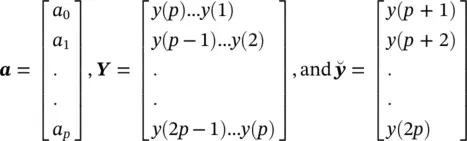

and a 0= 1. On the basis of (3.39), y ( n ) is calculated as the weighted sum of its p past values. y ( n ) is then constructed and the parameters f kand r kare estimated. Hence, the damping factors are obtained as

(3.46)

and the resonance frequencies as

(3.47)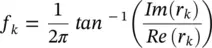

where Re(.) and Im(.) denote respectively the real and imaginary parts of a complex quantity. The w kparameters are calculated using the fact that 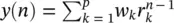or

(3.48)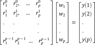

In vector form this can be illustrated as Rw= y, where k = 0, 1, ⋯, p − 1, l = 1, ⋯, p denoting the elements of the matrix in the above equation. Therefore, w= R −1 y, assuming R is a full‐rank matrix, i.e. there are no repeated poles. Often, this is simply carried out by implementing the Cholesky decomposition algorithm [34]. Finally, using w k, the amplitude and initial phases of the exponential terms are calculated as follows:

(3.49)

and

(3.50)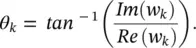

In the above solution we considered that the number of data samples N is equal to N = 2p , where p is the prediction order. For the cases where N > 2p a least‐squares (LS) solution for wcan be obtained as:

(3.51)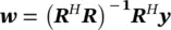

where (.) Hdenotes conjugate transpose. This equation can also be solved using the Cholesky decomposition method. For real data such as EEG signals this equation changes to w= ( R T R) −1 R T y, where (.) Trepresents the transpose operation. A similar result can be achieved using principal component analysis (PCA) [25].

In cases for which the data are contaminated with white noise, the performance of Prony's method is reasonable. However, for non‐white noise, the noise information is not easily separable from the data and therefore the method may not be sufficiently successful.

As we will see in a later chapter of this book, Prony's algorithm has been used in modelling and analysis of audio and visual EPs (AEP and VEP) [31, 35].

An approach similar to AR or MVAR modelling in which the output samples are nonlinearly related to the previous samples, may be followed based on the methods developed for forecasting financial growth in economical studies.

In the generalized autoregressive conditional heteroskedasticity (GARCH) method [36], each sample relates to its previous samples through a nonlinear (or sum of nonlinear) function(s). This model was originally introduced for time‐varying volatility (honoured with the Nobel Prize in Economic sciences in 2003).

Nonlinearities in the time series are declared with the aid of the McLeod and Li [37] and (Brock, Dechert, and Scheinkman) tests [38]. However, both tests lack the ability to reveal the actual kind of nonlinear dependency.

Generally, it is not possible to discern whether the nonlinearity is deterministic or stochastic in nature, nor can we distinguish between multiplicative and additive dependencies. The type of stochastic nonlinearity may be determined based on Hsieh test [39]. The additive and multiplicative dependencies can be discriminated by using this test. However, the test itself is not used to obtain the model parameters.

Considering the input to a nonlinear system to be u ( n ) and the generated signal as the output of such a system to be x ( n ), a restricted class of nonlinear models suitable for the analysis of such process is given by:

(3.52)

Multiplicative dependence means nonlinearity in the variance, which requires the function h (.) to be nonlinear; additive dependence, conversely, means nonlinearity in the mean, which holds if the function g (.) is nonlinear. The conditional statistical mean and variance are respectively defined as:

(3.53)

and

(3.54)

where χ n‐1contains all the past information up to time n ‐1. The original GARCH( p,q ) model, where p and q are the prediction orders, considers a zero mean case, i.e. g (.) = 0. If e ( n ) represents the residual (error) signal using the above nonlinear prediction system, we have:

(3.55)

where α jand β jare the nonlinear model coefficients. The second term (first sum) in the right side corresponds to a q th order moving average (MA) dynamical noise term and the third term (second sum) corresponds to an AR model of order p . It is seen that the current conditional variance of the residual at time sample n depends on both its previous sample values and previous variances.

Although in many practical applications such as forecasting of stock prices the orders p and q are set to small fixed values such as ( p,q ) = (1,1); for a more accurate modelling of natural signals such as EEGs the orders have to be determined mathematically. The prediction coefficients for various GARCH models or even the nonlinear functions g and h are estimated iteratively as for the linear ARMA models [36, 37].

Such simple GARCH models are only suitable for multiplicative nonlinear dependence. In addition, additive dependencies can be captured by extending the modelling approach to the class of GARCH‐M models [40].