Saeid Sanei - EEG Signal Processing and Machine Learning

Another limitation of the above simple GARCH model is failing to accommodate sign asymmetries. This is because the squared residual is used in the update equations. Moreover, the model cannot cope with rapid transitions such as spikes. Considering these shortcomings, numerous extensions to the GARCH model have been proposed. For example, the model has been extended and refined to include the asymmetric effects of positive and negative jumps such as the exponential GARCH model EGARCH [41], the GJR‐GARCH model [42], the threshold GARCH model (TGARCH) [43], the asymmetric power GARCH model APGARCH [44], and quadratic GARCH model QGARCH [45].

In these models different functions for g (.) and h (.) in (3.48)and (3.49)are defined. For example, in the EGARCH model proposed by Glosten et al. [41] h ( n ) is iteratively computed as:

(3.56)

where b , α 1, α 2, and κ are constants and η nis an indicator function that is zero when u nis negative and one otherwise.

Despite modelling the signals, the GARCH approach has many other applications. In some recent works [46] the concept of GARCH modelling of covariance is combined with Kalman filtering to provide a more flexible model with respect to space and time for solving the inverse problem. There are several alternatives for solution to the inverse problem. Many approaches fall into the category of constrained least‐squares methods employing Tikhonov regularization [47]. Among numerous possible choices for the GARCH dynamics, the EGARCH model [41] has been used to estimate the variance parameter of the Kalman filter iteratively.

Nonlinear models have not been used for EEG processing. To enable use of these models the parameters and even the order should be adapted to the EEG properties. Also, such a model should incorporate the changes in the brain signals due to abnormalities and onset of diseases.

In this very popular modelling approach the signals are characterized using the parameters of their distributions. The distributions in terms of probability density functions are sum of a number of Gaussian functions with different variances which are weighted and delayed differently [48]. The overall distribution subject to a set of K Gaussian components is defined as:

(3.57)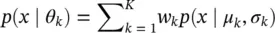

The vector of unknown parameters θ k= [ w k , μ k , σ k] for k = 1,2, …, K . w kis equivalent to the probability (weighting) that the data sample is generated by the k th mixture component density subject to:

(3.58)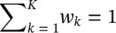

μ k, and σ kare mean and variances of the k th Gaussian distribution and p ( x | μ k, σ k) is a Gaussian function of x with parameters μ k, and σ k. Expectation maximization (EM) [49] is often used to estimate the above parameters by maximizing the log‐likelihood of the mixture of Gaussian (MOG) for an N ‐sample data defined as:

(3.59)

The EM algorithm alternates between updating the posterior probabilities used for generating each data sample by the k th mixture component (in a so‐called E‐step) as:

(3.60)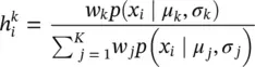

and weighted maximum likelihood updates of the parameters of each mixture component (in a so‐called M‐step) as:

(3.61)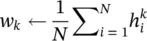

(3.62)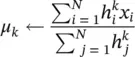

(3.63)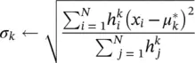

The EM algorithm (especially in cases of high‐dimensional multivariate Gaussian mixtures) may converge to spurious solutions when there are singularities in the log‐likelihood function due to small sample sizes, outliers, repeated data points or rank deficiencies leading to ‘variance collapse’. Some solutions to these shortcomings have been provided by many researchers such as those in [50–52]. Figure 3.13demonstrates how an unknown multimodal distribution can be estimated using weighted sum of Gaussians with different mean and variances:

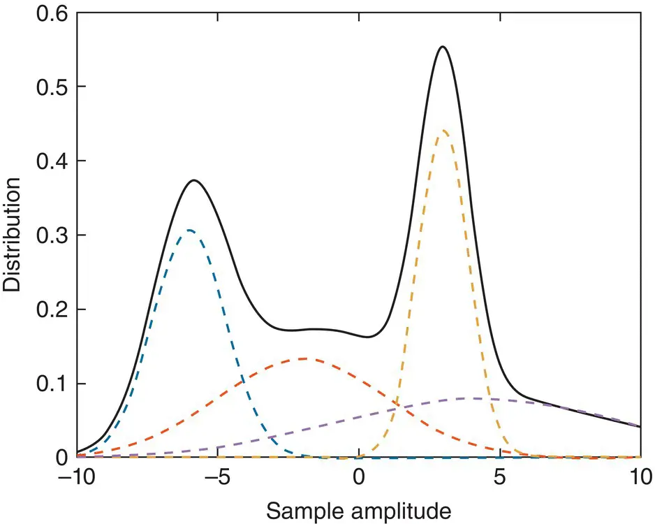
Figure 3.13 Mixture of Gaussian (dotted curves) models of a multimodal unknown distribution (bold curve).

Similar to prediction‐based models, the model order can be estimated using Akaike information criterion (AIC) or by iteratively minimizing the error for best model order. Also, mixture of exponential distributions can also be used instead of MOGs where there are sharp transients within the data. In [53] it has been shown that these models can be used for modelling variety of physiological data such as EEG, EOG, EMG, and ECG. In another work [54], the MOG model has been used for segmentation of magnetic resonance brain images. As a variant of the Gaussian mixture model (GMM), Bayesian GMMs have been used for partial amplitude synchronization detection in brain EEG signals [55]. This work introduces a method to detect subsets of synchronized channels that do not consider any baseline information. It is based on a Bayesian GMM applied at each location of a time–frequency map of the EEGs.

These models describe the cell as an independent unit. The well established models such as the Hodgkin–Huxley model have been implemented using electronic circuits. Although, for accurate models large numbers of components are required, in practise it has been shown that a good approximation of such models can be achieved using simple circuits [56].

Most of the models describing the excitation mechanism of the membrane are electronic realizations of the theoretical membrane model of Hodgkin and Huxley. In the following sections, two of these realizations are discussed.

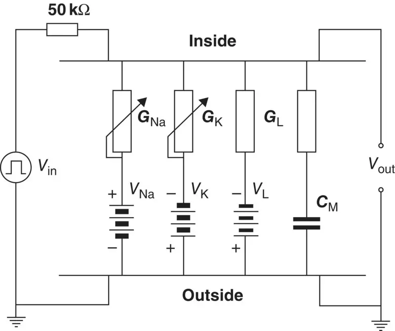
Figure 3.14 The Lewis membrane model [57].