Saeid Sanei - EEG Signal Processing and Machine Learning
Здесь есть возможность читать онлайн «Saeid Sanei - EEG Signal Processing and Machine Learning» — ознакомительный отрывок электронной книги совершенно бесплатно, а после прочтения отрывка купить полную версию. В некоторых случаях можно слушать аудио, скачать через торрент в формате fb2 и присутствует краткое содержание. Жанр: unrecognised, на английском языке. Описание произведения, (предисловие) а так же отзывы посетителей доступны на портале библиотеки ЛибКат.
- Название:EEG Signal Processing and Machine Learning
- Автор:
- Жанр:
- Год:неизвестен
- ISBN:нет данных
- Рейтинг книги:3 / 5. Голосов: 1
-
Избранное:Добавить в избранное
- Отзывы:
-
Ваша оценка:
EEG Signal Processing and Machine Learning: краткое содержание, описание и аннотация
Предлагаем к чтению аннотацию, описание, краткое содержание или предисловие (зависит от того, что написал сам автор книги «EEG Signal Processing and Machine Learning»). Если вы не нашли необходимую информацию о книге — напишите в комментариях, мы постараемся отыскать её.
EEG Signal Processing and Machine Learning — читать онлайн ознакомительный отрывок
Ниже представлен текст книги, разбитый по страницам. Система сохранения места последней прочитанной страницы, позволяет с удобством читать онлайн бесплатно книгу «EEG Signal Processing and Machine Learning», без необходимости каждый раз заново искать на чём Вы остановились. Поставьте закладку, и сможете в любой момент перейти на страницу, на которой закончили чтение.
Интервал:
Закладка:
(3.3) 
Then, for any perturbation of phase p ( ϕ ) this changes to [2]:
(3.4) 
(3.5) 
where:
(3.6) 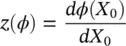
For a pair of oscillators of phases φ 1and φ 2, using the same analysis (see Figure 3.2, assuming p 12= p 21):
(3.7) 
(3.8) 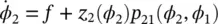
If it is further assumed that the phase difference φ 2− φ 1= φ changes slowly, then [2]:
(3.9) 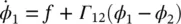
(3.10) 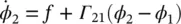
(3.11) 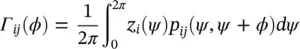
Γ ij( ϕ ) is called phase interaction function (PIF). Similarly, for N Rregions the rate of change of phase of the i th oscillator is given by:
(3.12) 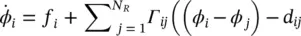
where f iis the intrinsic frequency of the i th oscillator. In these formulations there are two key assumptions: the first one is that the perturbations are sufficiently small that the differentiations can equivalently be evaluated at X 0rather than X . The second assumption is that the relative changes in the oscillator phase are sufficiently slow with respect to the oscillation frequency, that the phase offset term can be replaced by a time average.
In [2] an extension of the above WCO model is used to describe the dynamic phase changes in a network of oscillators. The use of Bayesian model comparison allows one to infer the mechanisms underlying synchronization processes in the brain. This has been applied to synthetic bimanual finger movement data from physiological models and on magnetoencephalogram (MEG) data from a study of visual working memory. The WCO approach accommodates signal nonstationarity by using differential equations which describe how the changes in phase are driven by pairwise differences in instantaneous phase.
3.2.3 Hodgkin–Huxley Model
Most probably the earliest physical model is based on the Hodgkin and Huxley's Nobel Prize winning mathematical model for a squid axon published in 1952 [8–10]. The Hodgkin and Huxley equations are important not only because they represent the most successful mathematical model in quantitatively describing the related biological phenomena but also due to the fact that deriving the model of a squid is directly applicable to many kinds of neurons and other excitable cells. According to this model, a nerve axon may be stimulated and the activated sodium (Na +) and potassium (K +) channels produced in the vicinity of the cell membrane can lead to the electrical excitation of the nerve axon. The excitation arises from the effect of the membrane potential on the movement of ions, and from interactions of the membrane potential with the opening and closing of voltage activated membrane channels. The membrane potential increases when the membrane is polarized with a net negative charge lining the inner surface and an equal but opposite net positive charge on the outer surface. This potential may be simply related to the amount of electrical charge Q , using:
(3.13) 
where Q is in terms of Coulombs cm −2, C mis the measure of the capacity of the membrane and has units farads cm −2and E has units of volts. In practise, in order to model the APs the amount of charge Q +on the inner surface (and Q −on the outer surface) of the cell membrane has to be mathematically related to the stimulating current I stimflowing into the cell through the stimulating electrodes. Figure 3.1b illustrates how the neuron excitation results in generation of APs by acting as a signal converter [11].
The electrical potential (often called electrical force) E is then calculated using Eq. (3.13). The Hodgkin and Huxley's model is illustrated in Figure 3.3. In this figure I membis the result of positive charges flowing out of the cell. This current consists of mainly three currents namely, Na, K, and leak currents. The leak current is due to the fact that the inner and outer Na and K ions are not exactly equal.
Hodgkin and Huxley estimated the activation and inactivation functions for the Na and K currents and derived a mathematical model to describe an AP similar to that of a giant squid. The model is a neuron model that uses voltage‐gated channels. The space‐clamped version of the Hodgkin–Huxley model may be well described using four ordinary differential equations [12]. This model describes the change in the membrane potential ( E ) with respect to time and is described in [13]. The overall membrane current is the sum of capacity current and ionic current as:
(3.14) 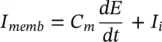
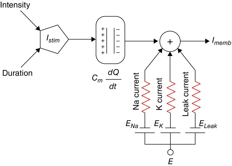
Figure 3.3 The Hodgkin–Huxley excitation model.
where I iis the ionic current and as indicated in Figure 3.1which can be considered as the sum of three individual components: Na, K, and leak currents:
(3.15) 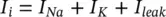
I Nacan be related to the maximal conductance  , activation variable a Na, inactivation variable h Na, and a driving force ( E – E Na) through:
(3.16) 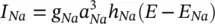
Интервал:
Закладка:
Похожие книги на «EEG Signal Processing and Machine Learning»
Представляем Вашему вниманию похожие книги на «EEG Signal Processing and Machine Learning» списком для выбора. Мы отобрали схожую по названию и смыслу литературу в надежде предоставить читателям больше вариантов отыскать новые, интересные, ещё непрочитанные произведения.


Обсуждение, отзывы о книге «EEG Signal Processing and Machine Learning» и просто собственные мнения читателей. Оставьте ваши комментарии, напишите, что Вы думаете о произведении, его смысле или главных героях. Укажите что конкретно понравилось, а что нет, и почему Вы так считаете.