Iain Pardoe - Applied Regression Modeling

Calculate test statistic: . (In most cases, this should be a positive number.)

Set significance level: %.

Look up critical value in Table C.1: The th percentile of the t‐distribution with degrees of freedom; the rejection region is any t‐statistic greater than this.

Make decision: If , then reject the null hypothesis in favor of the alternative. Otherwise, fail to reject the null hypothesis.

Interpret in the context of the situation: If we have rejected the null hypothesis in favor of the alternative, then the sample data suggest that a population mean of seems implausible—the sample data favor a value greater than this (at a significance level of %). If we have failed to reject the null hypothesis, then we have insufficient evidence to conclude that the population mean is greater than .

For a lower‐tail test, everything is the same except:

Alternative hypothesis: : .

In most cases, the should be a negative number.

Critical value: The th percentile of the t‐distribution with degrees of freedom; the rejection region is any t‐statistic less than this.

For a two‐tail test, everything is the same except:

Alternative hypothesis: : .

The could be positive or negative.

Critical value: The th percentile of the t‐distribution with degrees of freedom; the rejection region is any t‐statistic greater than this or less than the negative of this.

An alternative way to conduct a hypothesis test is to again assume initially that the null hypothesis is true, but then to calculate the probability of observing a t‐statistic as extreme as the one observed or even more extreme (in the direction that favors the alternative hypothesis). This is known as the p‐value (sometimes also called the observed significance level ):

1 – For an upper‐tail test, the p‐value is the area under the curve of the t‐distribution (with degrees of freedom) to the right of the observed t‐statistic.

2 – For a lower‐tail test, the p‐value is the area under the curve of the t‐distribution (with degrees of freedom) to the left of the observed t‐statistic.

3 – For a two‐tail test, the p‐value is the sum of the areas under the curve of the t‐distribution (with degrees of freedom) beyond both the observed t‐statistic and the negative of the observed t‐statistic.

If the p‐value is too “small,” then this suggests that it seems unlikely that the null hypothesis could have been true—so we reject it in favor of the alternative. Otherwise, the t‐statistic could well have arisen while the null hypothesis held true—so we do not reject it in favor of the alternative. Again, the significance level chosen tells us how small is small: If the p‐value is less than the significance level, then reject the null in favor of the alternative; otherwise, do not reject it. For the home prices example (see computer help #24 in the software information files available from the book website):

State null hypothesis: : .

State alternative hypothesis: : .

Calculate test statistic: .

Set significance level: 5%.

Look up p‐value: The area to the right of the t‐statistic (2.40) for the t‐distribution with 29 degrees of freedom is less than 0.025 but greater than 0.01 (since from Table C.1 the 97.5th percentile of this t‐distribution is 2.045 and the 99th percentile is 2.462); thus, the upper‐tail p‐value is between 0.01 and 0.025.

Make decision: Since the p‐value is between 0.01 and 0.025, it must be less than the significance level (0.05), so we reject the null hypothesis in favor of the alternative.

Interpret in the context of the situation: The 30 sample sale prices suggest that a population mean of seems implausible—the sample data favor a value greater than this (at a significance level of 5%).

To conduct an upper‐tail hypothesis test for a univariate mean using the p‐value method.

State null hypothesis: : .

State alternative hypothesis: : .

Calculate test statistic: . (In most cases, this should be a positive number.)

Set significance level: %.

Look up p‐value in Table C.1: Find which percentiles of the t‐distribution with degrees of freedom are either side of the t‐statistic; the p‐value is between the corresponding upper‐tail areas.

Make decision: If , then reject the null hypothesis in favor of the alternative. Otherwise, fail to reject the null hypothesis.

Interpret in the context of the situation: If we have rejected the null hypothesis in favor of the alternative, then the sample data suggest that a population mean of seems implausible—the sample data favor a value greater than this (at a significance level of %). If we have failed to reject the null hypothesis, then we have insufficient evidence to conclude that the population mean is greater than .

For a lower‐tail test, everything is the same except:

Alternative hypothesis: : .

In most cases, the should be a negative number.

p‐value: Find which percentiles of the t‐distribution with degrees of freedom are either side of the t‐statistic; the p‐value is between the corresponding lower‐tail areas.

For a two‐tail test, everything is the same except:

Alternative hypothesis: : .

The could be positive or negative.

p‐value: Find which percentiles of the t‐distribution with degrees of freedom are either side of the t‐statistic; p‐value/2 is between the corresponding upper‐tail areas (if the is positive) or lower‐tail areas (if the is negative). Thus, the p‐value is between the corresponding tail areas multiplied by two.

Figure 1.6shows why the rejection region method and the p‐value method will always lead to the same decision (since if the t‐statistic is in the rejection region, then the p‐value must be smaller than the significance level, and vice versa). Why do we need two methods if they will always lead to the same decision? Well, when learning about hypothesis tests and becoming comfortable with their logic, many people find the rejection region method a little easier to apply. However, when we start to rely on statistical software for conducting hypothesis tests in later chapters of the book, we will find the p‐value method easier to use. At this stage, when doing hypothesis test calculations by hand, it is helpful to use both the rejection region method and the p‐value method to reinforce learning of the general concepts. This also provides a useful way to check our calculations since if we reach a different conclusion with each method we will know that we have made a mistake.

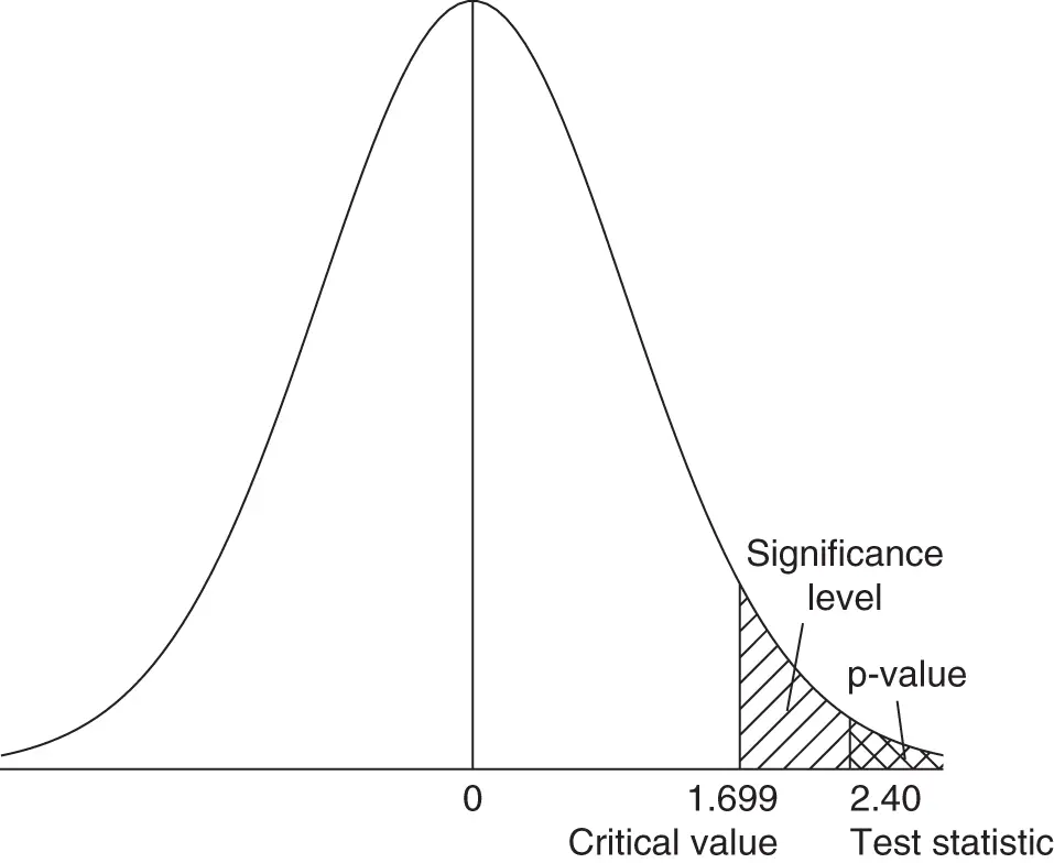
Figure 1.6Home prices example—density curve for the t‐distribution with degrees of freedom, together with the critical value of corresponding to a significance level of , as well as the test statistic of corresponding to a p‐value less than .

Lower‐tail tests work in a similar way to upper‐tail tests, but all the calculations are performed in the negative (left‐hand) tail of the t‐distribution density curve; Figure 1.7illustrates. A lower‐tail test would result in an inconclusive result for the home prices example (since the large, positive t‐statistic means that the data favor neither the null hypothesis, : , nor the alternative hypothesis, : ).