Scott D. Sudhoff - Power Magnetic Devices
Здесь есть возможность читать онлайн «Scott D. Sudhoff - Power Magnetic Devices» — ознакомительный отрывок электронной книги совершенно бесплатно, а после прочтения отрывка купить полную версию. В некоторых случаях можно слушать аудио, скачать через торрент в формате fb2 и присутствует краткое содержание. Жанр: unrecognised, на английском языке. Описание произведения, (предисловие) а так же отзывы посетителей доступны на портале библиотеки ЛибКат.
- Название:Power Magnetic Devices
- Автор:
- Жанр:
- Год:неизвестен
- ISBN:нет данных
- Рейтинг книги:4 / 5. Голосов: 1
-
Избранное:Добавить в избранное
- Отзывы:
-
Ваша оценка:
Power Magnetic Devices: краткое содержание, описание и аннотация
Предлагаем к чтению аннотацию, описание, краткое содержание или предисловие (зависит от того, что написал сам автор книги «Power Magnetic Devices»). Если вы не нашли необходимую информацию о книге — напишите в комментариях, мы постараемся отыскать её.
Discover a cutting-edge discussion of the design process for power magnetic devices Power Magnetic Devices: A Multi-Objective Design Approach
Power Magnetic Devices
Power Magnetic Devices — читать онлайн ознакомительный отрывок
Ниже представлен текст книги, разбитый по страницам. Система сохранения места последней прочитанной страницы, позволяет с удобством читать онлайн бесплатно книгу «Power Magnetic Devices», без необходимости каждый раз заново искать на чём Вы остановились. Поставьте закладку, и сможете в любой момент перейти на страницу, на которой закончили чтение.
Интервал:
Закладка:
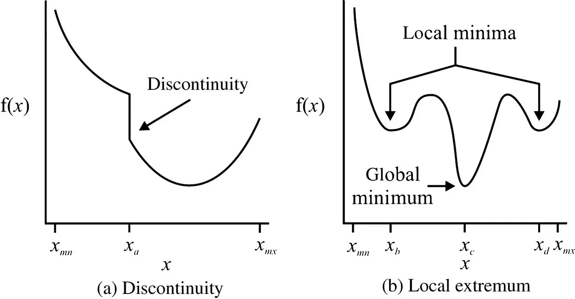
Figure 1.3 Function properties.
Another property that can be problematic is the existence of local minima. These are illustrated in Figure 1.3(b). Therein x = x b, x = x c, and x = x dare all local minima; however, only the point x = x cis a global minimizer. Many minimization algorithms can converge to local minimizers and fail to find the global minimizer.
Related to the existence of local extrema is the convexity (or lack thereof) of a function. It is appropriate to begin the discussion of function convexity by considering the definition of a convex set. Let Θ ⊂ ℝ ndenote a set. A set is considered convex if all the points on the line connecting any two points in the set are also in the set. In other words, if
(1.2-2) 
for any two points x a, x b∈ Θ then Θ is convex. This is illustrated in Figure 1.4for Θ ⊂ ℝ 2.
In order to determine if a function is convex, it is necessary to consider its epigraph. The epigraph of f( x) is simply the set of points greater than or equal to f( x). A function is considered convex if its epigraph is a convex set, as is shown in Figure 1.5. Note that this set will be in ℝ n + 1, where n is the dimension of x.
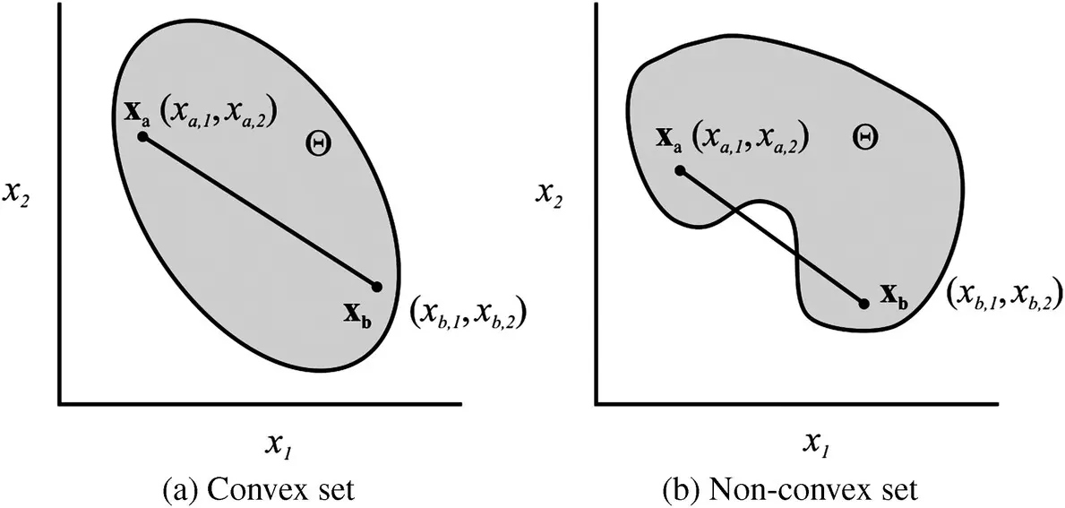
Figure 1.4 Definition of a convex set.
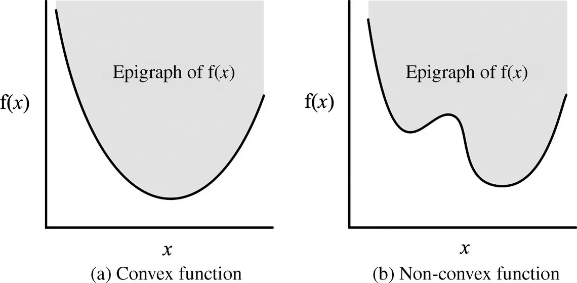
Figure 1.5 Definition of a convex function.
If the function being optimized is convex, the optimization process becomes much easier. This is because it can be shown that any local minimizer of a convex function is also a global minimizer. Therefore the situation shown in Figure 1.3(b) cannot occur. As a result, the minimization of continuous convex functions is straightforward and computationally tractable.
1.3 Single‐Objective Optimization Using Newton’s Method
Let us consider a method to find the extrema of an objective function f( x). Let us focus our attention on the case where f( x) ∈ ℝ and x∈ ℝ n. Algorithms to solve this problem include gradient methods, Newton’s method, conjugate direction methods, quasi‐Newton methods, and the Nelder–Mead simplex method, to name a few. Let us focus on Newton’s method as being somewhat representative.
In order to set the stage for Newton’s method, let us first define some operators. The first derivative or gradient of our objective function is denoted ∇f( x) and is defined as
(1.3-1) 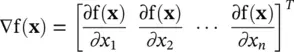
The second derivative or Hessian of f( x)is defined as
(1.3-2) 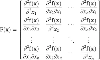
If x *is a local minimizer of f, and if x *is in the interior of Ω, it can be shown that
(1.3-3) 
and that
(1.3-4) 
Note that the statement F( x *) ≥ 0 means that F( x *) is positive semi‐definite, which is to say that y TF( x *) y≥ 0 ∀ y∈ ℝ n. This second condition verifies that a minimum rather than a maximum has been found. It is important to understand that the conditions (1.3-3)and (1.3-4)are necessary but not sufficient conditions for x *to be a mimimizer, unless f is a convex function. If f is convex, (1.3-3)and (1.3-4)are necessary and sufficient conditions for x *to be a global minimizer.
At this point, we are posed to set forth Newton’s method of finding function minimizers. This method is iterative and is based on a k th estimate of the solution denoted x[ k ]. Then an update formula is applied to generate a (hopefully) improved estimate x[ k + 1] of the minimizer. The update formula is derived by first approximating f as a Taylor series about the current estimated solution x[ k ]. In particular,
(1.3-5) 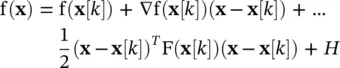
where H denotes higher‐order terms. Neglecting these higher‐order terms and finding the gradient of f( x) based on (1.3-5), we obtain
(1.3-6) 
From the necessary condition (1.3-3), we next take the right‐hand side of (1.3-6)and equate it with zero; then we replace x, which will be our improved estimate, with x[ k + 1]. Manipulating the resulting expression yields
(1.3-7) 
which is Newton’s method.
Clearly, Newton’s method requires f ⊂ C 2, which is to say that f is in the set of twice differentiable functions. Note that the selection of the initial solution, x[1], can have a significant impact on which (if any) local solution is found. Also note that method is equally likely to yield a local maximizer as a local minimizer.
Example 1.3A
Let us apply Newton’s method to find the minimizer of the function
(1.3A-1) 
This example is an arbitrary mathematical function; we will consider how to construct f( x) so as to serve a design purpose in Section 1.9. Inspection of (1.3A-1)reveals that the global minimum is at x 1= 2 and x 2= ln (2). However, let us apply Newton’s method to find the minimum. Our first step is to obtain the gradient and the Hessian. From (1.3A-1), we have
(1.3A-2) 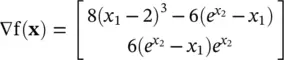
Интервал:
Закладка:
Похожие книги на «Power Magnetic Devices»
Представляем Вашему вниманию похожие книги на «Power Magnetic Devices» списком для выбора. Мы отобрали схожую по названию и смыслу литературу в надежде предоставить читателям больше вариантов отыскать новые, интересные, ещё непрочитанные произведения.


Обсуждение, отзывы о книге «Power Magnetic Devices» и просто собственные мнения читателей. Оставьте ваши комментарии, напишите, что Вы думаете о произведении, его смысле или главных героях. Укажите что конкретно понравилось, а что нет, и почему Вы так считаете.