Computational Statistics in Data Science

Before providing two recent examples of twenty‐first century computational statistics ( Section 3), we present three easily quantified Core Challenges within computational statistics that we believe will always exist: big , or inference from many observations; big , or inference with high‐dimensional models; and big , or inference with nonconvex objective – or multimodal density – functions. In twenty‐first century computational statistics, these challenges often co‐occur, but we consider them separately in this section.

Having a large number of observations makes different computational methods difficult in different ways. A worst case scenario, the exact permutation test requires the production of datasets. Cheaper alternatives, resampling methods such as the Monte Carlo permutation test or the bootstrap, may require anywhere from thousands to hundreds of thousands of randomly produced datasets [8, 10]. When, say, population means are of interest, each Monte Carlo iteration requires summations involving expensive memory accesses. Another example of a computationally intensive model is Gaussian process regression [16, 17]; it is a popular nonparametric approach, but the exact method for fitting the model and predicting future values requires matrix inversions that scale . As the rest of the calculations require relatively negligible computational effort, we say that matrix inversions represent the computational bottleneck for Gaussian process regression.

To speed up a computationally intensive method, one only needs to speed up the method's computational bottleneck. We are interested in performing Bayesian inference [18] based on a large vector of observations . 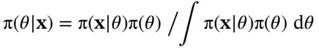We specify our model for the data with a likelihood function and use a prior distribution with density function to characterize our belief about the value of the ‐dimensional parameter vector a priori . The target of Bayesian inference is the posterior distribution of conditioned on

(1)

The denominator's multidimensional integral quickly becomes impractical as grows large, so we choose to use the MetropolisHastings (M–H) algorithm to generate a Markov chain with stationary distribution [19, 20]. We begin at an arbitrary position and, for each iteration , randomly generate the proposal state from the transition distribution with density . We then accept proposal state with probability

(2)

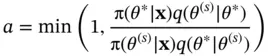
The ratio on the right no longer depends on the denominator in Equation (1), but one must still compute the likelihood and its terms .

It is for this reason that likelihood evaluations are often the computational bottleneck for Bayesian inference. In the best case, these evaluations are , but there are many situations in which they scale [21, 22] or worse. Indeed, when is large, it is often advantageous to use more advanced MCMC algorithms that use the gradient of the log‐posterior to generate better proposals. In this situation, the log‐likelihood gradient may also become a computational bottleneck [21].

One of the simplest models for big problems is ridge regression [23], but computing can become expensive even in this classical setting. Ridge regression estimates the coefficient by minimizing the distance between the observed and predicted values and along with a weighted square norm of :