Computational Statistics in Data Science

Confidence intervals are notoriously difficult to understand at a first instance, and thus a standard Monte Carlo experiment in an introductory statistics course is that of repeating the above experiment multiple times and illustrating that on average about proportion of such confidence intervals will contain the true mean. That is, for , we generate 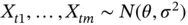, calculate the mean and the sample variance , and define to be

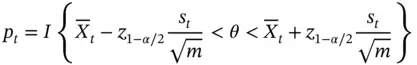
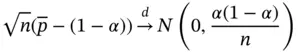
where is the indicator function. By the law of large numbers, 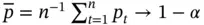with probability 1, as , and the following CLT holds:

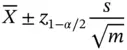
In conducting this experiment, we must choose the Monte Carlo sample size . A reasonable argument here is that our estimator must be accurate up to the second significant digit with roundoff. That is, we may allow a margin of error of 0.005. This implies that must be chosen so that

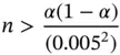
That is, to construct, say a confidence interval, an accurate Monte Carlo study in this simple example requires at least 1900 Monte Carlo samples. A higher precision would require an even larger simulation size! This is an example of an absolute precision stopping rule ( Section 5) and is unique since the limiting variance is known. For further discussion of this example, see Frey [8].

Recall that is a ‐dimensional target distribution, and interest is in estimating different features of . In Monte Carlo simulation, we generate either via IID sampling or via a Markov chain that has as its limiting distribution. For MCMC samples, we assume throughout that a Harris ergodic Markov chain is employed ensuring convergence of sample statistics to (finite) population quantities (see Roberts and Rosenthal [9], for definitions).

The most common quantity of interest in Monte Carlo simulations is the expectation of a function of the target distribution. Let denote the Euclidean norm, and let , so that interest is in estimating

where we assume . If is identity, then the mean of the target is of interest. Alternatively, can be chosen so that moments or other quantities are of interest. A Monte Carlo estimator of is

For IID and MCMC sampling, the ergodic theorem implies that as . The Monte Carlo average is naturally unbiased as long as the samples are either IID or the Markov chain is stationary.

Quantiles are particularly of interest when making credible intervals in Bayesian posterior distributions or making boxplots from Monte Carlo simulations. In this section, we assume that is one‐dimensional (i.e., ). Extensions to are straightforward but notationally involved [10]. For , interest may be in estimating a quantile of . Let be the distribution function of , assumed to be absolutely continuous with a continuous density . The ‐quantile associated with is