Computational Statistics in Data Science

110 110 Wei, X., Liu, Y., Wanga, X. et al. (2019) A survey on quality‐assurance approximate stream processing and applications. Futur. Gener. Comput. Syst., 101, 1062–1080.

111 111 Quoc, D.L., Krishnan, D.R., Bhatotia, P. et al. (2018) Incremental approximate computing, in Encyclopedia of Big Data Technologies (eds S. Sakr and A. Zomaya), Springer, Cham.

112 112 Sigurleifsson, B., Anbarasu, A., and Kangur, K. (2019) An overview of count‐min sketch and its application. EasyChair, 879, 1–7.

113 113 Garofalakis, M., Gehrke, J., and Rastogi, R. (eds) (2016) Data Stream Management: Processing High‐Speed Data Streams, Springer, Berlin, Heidelberg.

114 114 Sakr, S. (2016) Big Data 2.0 Processing Systems: A Survey, Springer, Switzerland. doi: 10.1007/978‐3‐319‐38776‐5.

115 115 Yates, J. (2020) Stream Processing with IoT Data: Challenges, Best Practices, and Techniques, https://www.confluent.io/blog/stream‐processing‐iot‐data‐best‐practices‐and‐techniques.

116 116 Zhao, X., Garg, S., Queiroz, C., and Buyya, R. (2017) A taxonomy and survey of stream processing systems, in Software Architecture for Big Data and the Cloud (eds I. Mistrik, R. Bahsoon, N. Ali, et al.), Elsevier, pp. 183–206. doi: 10.1016/B978‐0‐12‐805467‐3.00011‐9.

117 117 Landset, S., Khoshgoftaar, T.M., Richter, A.N., and Hasanin, T. (2015) A survey of open source tools for machine learning with big data in the Hadoop ecosystem. J. Big Data, 2 (1), 1–36.

Dootika Vats1, James M. Flegal2, and Galin L. Jones3

1Indian Institute of Technology Kanpur, Kanpur, India

2University of California, Riverside, CA, USA

3University of Minnesota, Twin‐Cities Minneapolis, MN, USA

Monte Carlo simulation methods generate observations from a chosen distribution in an effort to estimate unknowns of that distribution. A rich variety of methods fall under this characterization, including classical Monte Carlo simulation, Markov chain Monte Carlo (MCMC), importance sampling, and quasi‐Monte Carlo.

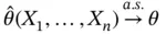
Consider a distribution defined on a ‐dimensional space , and suppose that are features of interest of . Specifically, may be a combination of quantiles, means, and variances associated with . Samples are obtained via simulation either approximately or exactly from , and a consistent estimator of , , is constructed so that, as ,

(1)

Thus, even when is a complicated distribution, Monte Carlo simulation allows for estimation of features of . Throughout, we assume that either independent and identically distributed (IID) samples or MCMC samples from can be obtained efficiently; see Refs [1–5] for various techniques.

The foundation of Monte Carlo simulation methods rests on asymptotic convergence as indicated by ( 1). When enough samples are obtained, , and simulation can be terminated with reasonable confidence. For many estimators, an asymptotic sampling distribution is available in order to ascertain the variability in estimation via a central limit theorem (CLT) or application of the delta method on a CLT. Section 2introduces estimators of , while Section 3discusses sampling distributions of these estimators for IID and MCMC sampling.

Although Monte Carlo simulation relies on large‐sample frequentist statistics, it is fundamentally different in two ways. First, data is generated by a computer, and so often there is little cost to obtaining further samples. Thus, the reliance on asymptotics is reasonable. Second, data is obtained sequentially, so determining when to terminate the simulation can be based on the samples already obtained. As this implies a random simulation time, additional safeguards are necessary to ensure asymptotic validity. This has led to the study of sequential stopping rules, which we present in Section 5.

Sequential stopping rules rely on estimating the limiting Monte Carlo variance–covariance matrix (when , this is the standard error of ). This is a particularly challenging problem in MCMC due to serial correlation in the samples. We discuss these challenges in Section 4and present estimators appropriate for large simulation sizes.

Over a variety of examples in Section 7, we conclude that the simulation size required for a reliable estimation is often higher than what is commonly used by practitioners (see also Refs [6, 7]. Given modern computational power, the recommended strategies can easily be adopted in most estimation problems. We conclude the introduction with an example illustrating the need for careful sample size calculations.

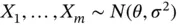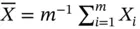Example 1. Consider IID draws . An estimate of is , and is estimated with the sample variance, . Let be the th quantile of a standard normal distribution, for . A large‐sample confidence interval for is