Bioinformatics and Medical Applications

K means, an unsupervised algorithm, endeavors to iteratively segment the dataset into K pre-characterized and nonoverlapping data groups with the end goal that one data point can have a place with just one bunch. It attempts to make the intra-group data as similar as could reasonably be expected while keeping the bunches as various (far) as could be expected under the circumstances. It appoints data points to a cluster with the end goal that the entirety of the squared separation between the data points and the group’s centroid is at the minimum. The less variety we have inside bunches, the more homogeneous the data points are inside a similar group.

Ensemble method is the process by which various models are created and consolidated in order to understand a specific computer intelligence problem. This prompts better prescient performance than could be acquired from any of the constituent learning models alone. Fundamentally, an ensemble is a supervised learning method for joining various weak learners/models to deliver a strong learner. Ensemble model works better, when we group models with low correlation. Figure 1.7gives the various ensemble methods which are in use. Following are some of the techniques used for ensemble.

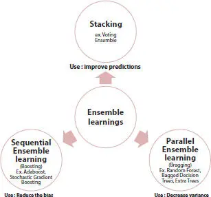
Figure 1.7 Ensemble methods.

Bagging or bootstrap aggregation assigns equal weights to each model in the ensemble. It trains each model of the ensemble separately using random subset of training data in order to promote variance. Random Forest is a classical example of bagging technique where multiple random decision trees are combined to achieve high accuracy. Samples are generated in such a manner that the samples are different from each other and replacement is permitted.

The term “Boosting” implies a gathering of calculations which changes a weak learner to strong learner. It is an ensemble technique for improving the model predictions of some random learning algorithm. It trains weak learners consecutively, each attempting to address its predecessor. There are three kinds of boosting in particular, namely, AdaBoost that assigns more weight to the incorrectly classified data that would be passed on to the next model, Gradient Boosting which uses the residual errors made by previous predictor to fit the new predictor, and Extreme Gradient Boosting which overcomes drawbacks of Gradient Boosting by using parallelization, distributed computing, out-of-core computing, and cache optimization.

It utilizes meta-learning calculations to discover how to join the forecasts more readily from at least two basic algorithms. A meta model is a two-level engineering with Level 0 models which are alluded to as base models and Level 1 model which are alluded to as Meta model. Meta-model depends on forecasts made by basic models on out of sample data. The yields from the base models utilized as contribution to the meta-model might be in the form of real values in the case of regression and probability values in the case of classification. A standard method for setting up a meta-model training database is with k-fold cross-validation of basic models.

Each model makes a forecast (votes) in favor of each test occurrence and the final output prediction is the one that gets the greater part of the votes. Suppose for a specific order issue we are given three diverse classification rules, c 1(X); c 2(X); c 3(X), we join these rules by majority voting as

Naive Bayes multi-model decision-making system, which is our proposed method uses ensemble method of type majority voting using a combination of Naive Bayes, Decision Tree, and Random Forest for analytics in the database of heart disease patients and attains an accuracy that outperforms any of the individual methods. Additionally, it uses K means along with the combination of the above methods for further increase the accuracy.

The data pertains to Kaggle dataset for cardiovascular disease which contains 12 attributes. Whether or not cardiovascular disease is present is contained in column carrying target value which is a binary type having values 0 and 1 indicating absence or presence respectively. There are a total of 70,000 records having attributes for age, tallness, weight, gender, systolic and diastolic blood pressure, cholesterol, glucose, smoking, alcohol intake, and physical activity.

Training and testing data is divided in the ratio 70:30. During training and testing, we tried various combinations to see their effect of accuracy of predictions. Also, we took data in chunks of 1000, 5000, 10,000, 50,000 and 70,000, respectively, and observed the change in patterns. We tried various combinations to check on the accuracy.

• NB: Only Naive Bayes algorithm is applied.

• DT: Only Decision Tree algorithm is applied.

• RF: Only Random Forest algorithm is applied.

• Serial: Naive Bayes followed by Random Forest followed by Decision tree (in increasing order of individual accuracy).

• Parallel: All three algorithms are applied in parallel and maximum voting is used.

• Prob 60 SP: If probability calculated by Naive Bayes is greater than 60% apply serial method else apply parallel.

• PLS: First parallel then serial is applied for wrong classified records.

• SKmeans: Combination of Serial along with K means.

• PKmeans: Combination of Parallel along with K means.

From this analysis, we found the PKmeans method to be the most efficient. Though serial along with K means achieves the best accuracy for training data, it is not feasible for real data where target column is not present. The reliability on any single algorithm is not possible for correctly classifying all the records; hence, we use more suitable ensemble method which utilizes the wisdom of the crowd. It uses the ensemble method of the type majority voting which includes adding the decisions in favor of crisp class labels from different models and foreseeing the class with the most votes.

Our goal is to achieve the best possible accuracy which surpasses the accuracy achieved by the individual methods. Figures 1.8to 1.11show the confusion matrix plotted by Naive Bayes, Random Forest, and Decision Tree individually as well as their ROC curve.

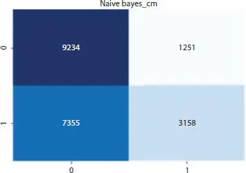
Figure 1.8 NB confusion matrix.

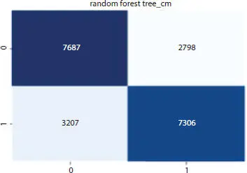
Figure 1.9RF confusion matrix.

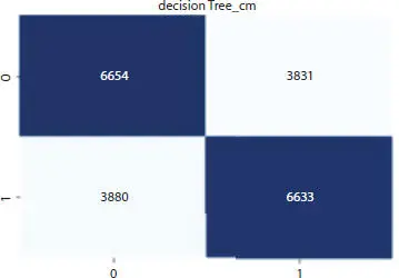
Figure 1.10DT confusion matrix.

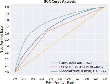
Figure 1.11 ROC curve analysis.