Anthony R. West - Solid State Chemistry and its Applications

The face centred lattice, F, contains additional lattice points in the centre of each face (c). An example of a face centred cubic, fcc, structure is Cu metal. A side centred lattice contains extra lattice points on only one pair of opposite faces. It is labelled a C‐centred lattice if the extra lattice points are on the ab face of the unit cell, as in (d). Similarly, an A‐centred lattice has lattice points on the bc face.

A body centred lattice, I, has an extra lattice point at the body centre (e). α ‐Iron is body centred cubic, bcc, because it has a cubic unit cell with Fe atoms at the corner and body centre positions.

CsCl is also cubic with Cs at corners and Cl at the body centre (or vice versa), but it is primitive, P. This is because, for a lattice to be body centred, the atom or group of atoms located at or near the corner must be identical with those at or near the body centre.

In the simplest cases of monatomic metals such as Cu and α ‐Fe, mentioned above, the arrangement of metal atoms in the structure is simply the same as the arrangement of lattice points. In more complex structures such as NaCl, the lattice point represents an ion pair. This is still a very simple example, however, and in most inorganic structures the lattice point represents a considerable number of atoms. In crystals of organic molecules such as proteins, the lattice point represents an entire protein molecule. Obviously the lattice point gives no information whatsoever as to the atoms and their arrangements which it represents; what the lattice does show is how these species are packed together in 3D.

The combination of crystal system and lattice type gives the Bravais lattice of a structure. There are 14 possible Bravais lattices. They are given in Table 1.1, and shown in Fig. 1.12, by combining crystal system, column 1 and lattice type, column 4. For example, P‐monoclinic, C‐centred monoclinic and P‐triclinic are three of the 14 possible Bravais lattices. The lattice type plus unit cell combinations which are absent either (a) would violate symmetry requirements, e.g. a C‐centred lattice cannot be cubic because it would not have the necessary threefold axes or (b) may be represented by a smaller, alternative cell, e.g. a face centred tetragonal cell can be redrawn as a body centred tetragonal cell; the symmetry is still tetragonal but the volume is halved, Fig. 1.10(b).

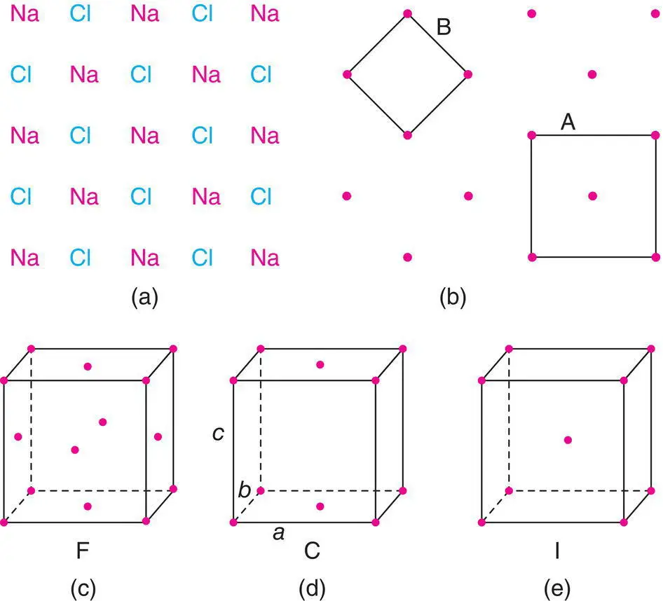
Figure 1.11 Representation of (a) the NaCl structure in two dimensions by (b) an array of lattice points; (c) face centred, (d) side centred and (e) body centred lattices.

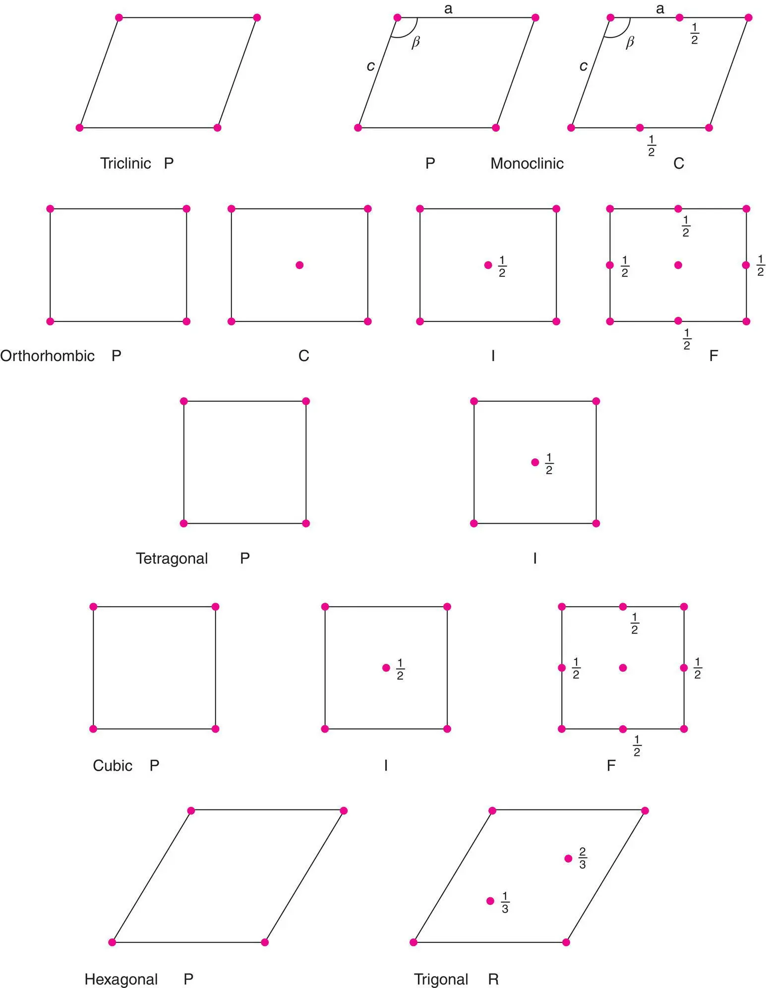
Figure 1.12 The unit cells of the 14 Bravais lattices: axes refer to the ab plane, unless specified. Heights of lattice points are 0, 1, unless specified.

D. McKie and C. McKie, Essentials of Crystallography, John Wiley & Sons (1986).

The concept of lattice planes causes considerable confusion because there are two separate ideas which can easily become mixed. Any simple structure, such as a metal or an ionic structure, may, in certain orientations, be regarded as built of layers or planes of atoms stacked to form a 3D structure. These layers are often related in a simple manner to the unit cell; for example, a unit cell face may coincide with a layer of atoms. The reverse is not necessarily true, however, especially in more complex structures and unit cell faces or simple sections through the unit cell often do not coincide with layers of atoms in the crystal. Lattice planes, a concept introduced with Bragg's law of diffraction ( Chapter 5), are defined purely from the shape and dimensions of the unit cell. Lattice planes are entirely imaginary and simply provide a reference grid to which the atoms in the crystal structure may be referred. Sometimes, a given set of lattice planes coincides with layers of atoms, but not usually.

Consider the 2D array of lattice points shown in Fig. 1.13(a). This array may be divided into many different sets of rows and for each set there is a characteristic perpendicular distance, d , between pairs of adjacent rows. In three dimensions, these rows become lattice planes and adjacent planes are separated by the interplanar d‐spacing, d . (Bragg's law treats X‐rays as being diffracted from these various sets of lattice planes and the Bragg diffraction angle, θ , for each set is related to the d ‐spacing by Bragg's law.)

Lattice planes are labelled by assigning three numbers known as Miller indices to each set. The derivation of Miller indices is illustrated in Fig. 1.13(b) (and those for a hexagonal lattice are shown in Fig. 1.14). The origin of the unit cell is at point 0. Two planes are shown which are parallel and pass obliquely through the unit cell. A third plane in this set must, by definition, pass through the origin. Each of these planes continues out to the surface of the crystal and in so doing cuts through many more unit cells; also, there are many more planes in this set parallel to the two shown, but which do not pass through this particular unit cell.

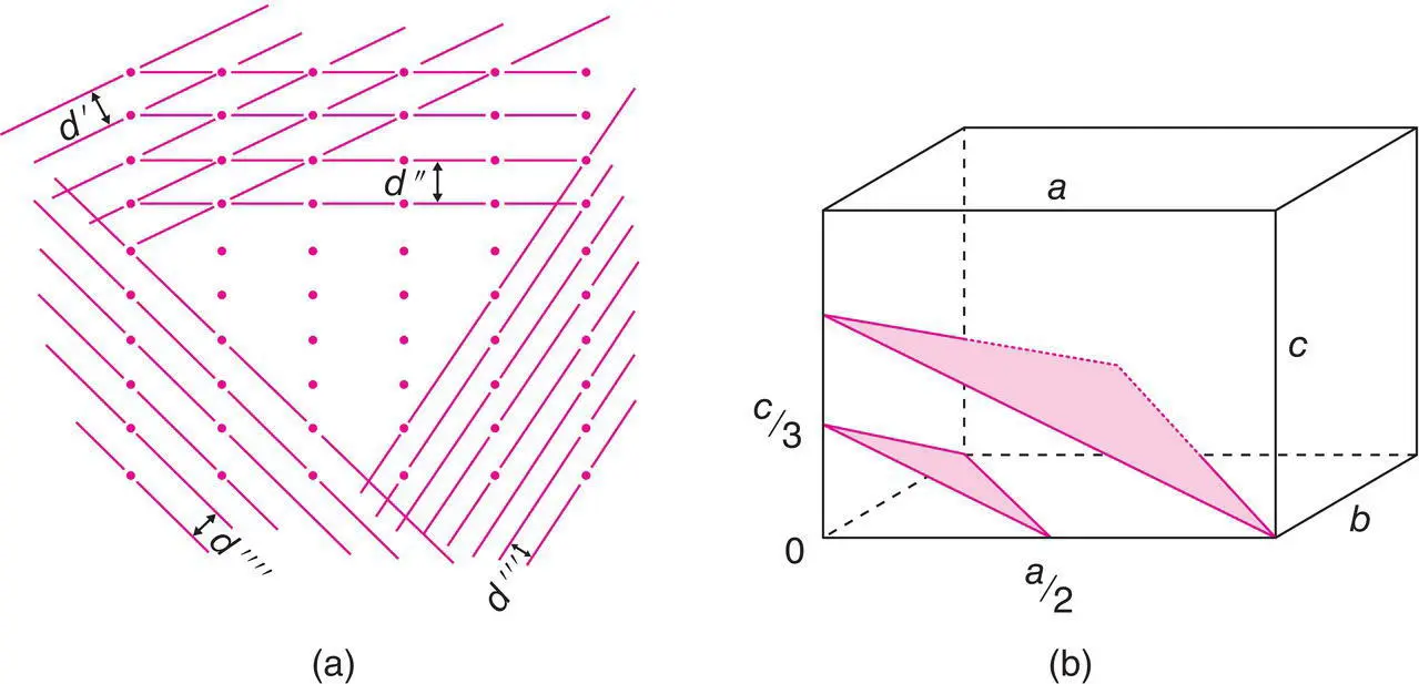
Figure 1.13 (a) Lattice planes (in projection); (b) derivation of Miller indices.

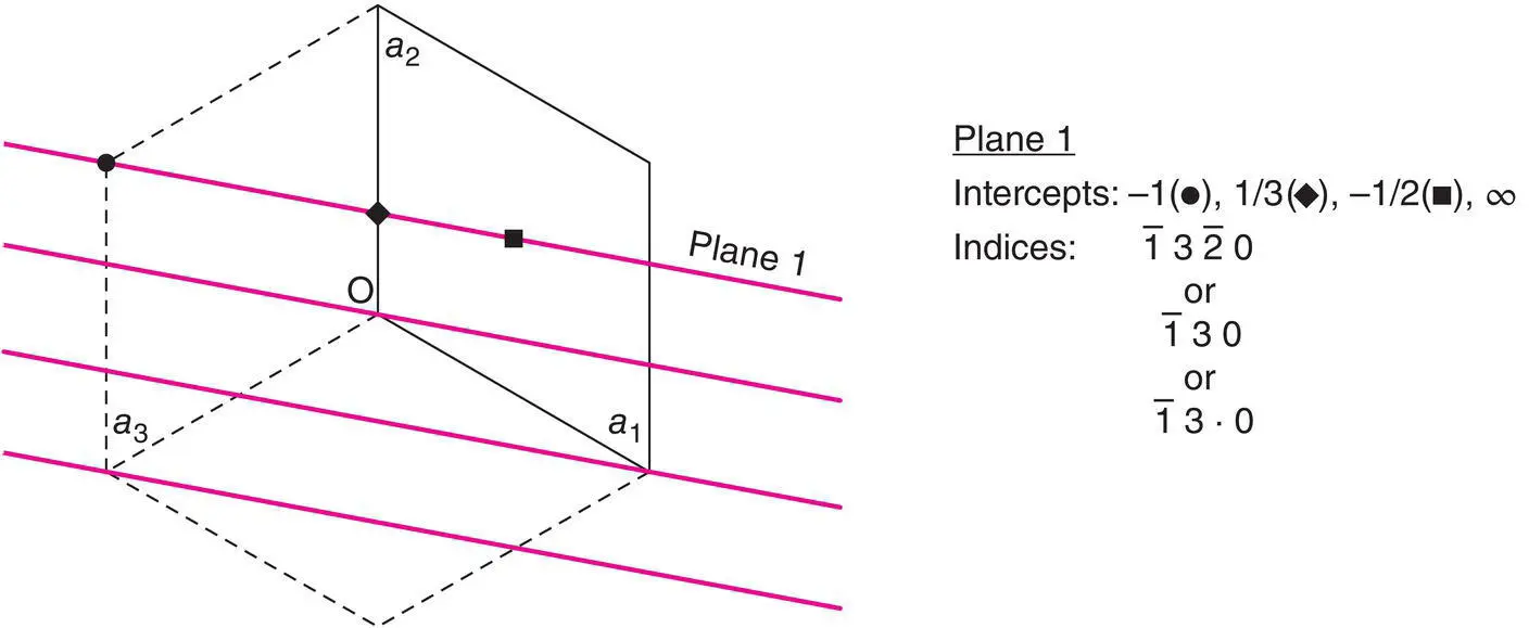
Figure 1.14 Miller indices for a hexagonal lattice.

In order to assign Miller indices to a set of planes, there are four stages:

1 From the array of lattice points, or the crystal structure, identify the unit cell, choose the origin and label the axes a, b, c and angles α (between b and c), β (between a and c) and γ (between a and b).

2 For a particular set of lattice planes, identify that plane which is adjacent to the one that passes through the origin.

3 Find the intersection of this plane on the three axes of the cell and write these intersections as fractions of the cell edges. The plane in question, Fig. 1.13(b), cuts the x axis at a/2, the y axis at b and the z axis at c/3; the fractional intersections are therefore ½, 1, ⅓.

4 Take reciprocals of these fractions and write the three numbers in parentheses; this gives (213). These three integers, (213), are the Miller indices of the plane and all other planes parallel to it and separated from adjacent planes by the same d‐spacing.

Some other examples are shown in Fig. 1.15. In (a), the shaded plane cuts x , y and z at 1 a , ∞ b and 1 c , i.e. the plane is parallel to b . Taking reciprocals of 1, ∞ and 1 gives us (101) for the Miller indices. A Miller index of 0 means, therefore, that the plane is parallel to that axis. In Fig. 1.15(b), the planes of interest comprise opposite faces of the unit cell. We cannot determine directly the indices of plane 1 as it passes through the origin. Plane 2 has intercepts of 1 a , ∞ b and ∞ C and Miller indices of (100).

Figure 1.15(c) is similar to (b) but there are now twice as many planes as in (b). To find the Miller indices, consider plane 2, which is the one that is closest to the origin but without passing through it. Its intercepts are ½, ∞ and ∞ and the Miller indices are (200). A Miller index of 2, therefore indicates that the plane cuts the relevant axis at half the cell edge. This illustrates an important point. After taking reciprocals, do not divide through by the highest common factor. A common source of error is to regard, say, the (200) set of planes as those planes interleaved between the (100) planes, to give the sequence (100), (200), (100), (200), (100), …. The correct labelling is shown in Fig. 1.15(d). If extra planes are interleaved between adjacent (100) planes then all planes are labelled as (200).