Rethinking Prototyping

The projection method and constraint force method are integrated into our scheme. The projection method is applied to find grid patterns that exactly fulfil the geometric constraints, while the constraint force method allows the obtained forms to deviate from the target surfaces. The fitness of the obtained forms to the target surfaces is controlled by the magnitude of constraint forces. Smaller constraint forces, which result in less fitness, generate grid patterns that exhibit lower strain energy.

The profile stiffness can be used as an active factor in the form-finding process. The real stiffness (a profile stiffness of a practical profile that can be used in the bearing structure) is useful to explore the structural behaviour of elastic grids under geometric constraints. Besides, the real stiffness facilitates the form-finding of a grid pattern in accordance with the pre-determined grid lengths. Meanwhile, the fictitious stiffness (a profile stiffness that is designed on purpose and is only used in the form-finding stage) enables the grids to have a larger range of strained lengths, which facilitates the reduction of bending stresses and can be utilised to generate smoothly curved grid patterns with various grid lengths.

Jian-Min Li, Jan Knippers

Institute of Building Structures and Structural Design (ITKE), University of Stuttgart, Germany

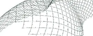
Fig. 1 Structural model of a single-layer grid shell with equal grid lengths

The rest of the article is structured as follows: In Sec. 2, we describe the structural modelling of elastic beams. In Sec. 3, we illustrate how to apply geometric constraints. In Sec. 4, four examples are given. In the final section, our conclusions are provided.

Our beam model is visualised as two separated nodes/particles with an interval as the beam length and each node is assigned a mass term and an inertia term. The nodes will shift and rotate freely if no force or torque is exerted. Once the internal forces are applied, the nodal movements become coupled and the individual nodes will behave as an integral structure.

DR is an explicit time integration method [6], which is applied in our scheme to simulate the above-mentioned system. With the information of the state of the previous time step and the forces currently exerted on the system, we can calculate the state of the subsequent time step.

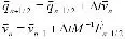
Translational motion is described by nodal positions and translational velocities, while rotational motion is described by nodal orientations and angular velocities. The rates of change of translational velocities and rotational velocities are proportional to the residuals of translational forces and torques exerted on nodes. The update formulations for translation motion and rotational motion are listed in Tab. 1. The derivation and the application of these formulations are illustrated in our previous work.

Table 1: Translation and rotation formulations of DR
Translational part	Rotational part

With proper damping, the kinetic energy is reduced to zero and a static state can be derived. We use two different damping methods: For the translational degrees of freedom we use kinetic damping, setting every translational velocity to zero once the translational kinetic energy of the system begins to decrease. For the rotational degrees of freedom we use velocity damping, multiplying every angular velocity by a factor less than one at each time step [7].

To calculate the internal forces in beam elements, we need to define additional orientations of the beam-ends. In this paper, we consider only rigid joints. That means each beam end will rotate simultaneously with the corresponding node and maintain their relative difference in orientations. The Euler-Bernoulli beam element, which has 12 DOF each, is used to calculate internal forces in beams. The axial force, bending moments and torque are determined by the corresponding positions and orientations of the two beam-ends of the beam element. The formulations for calculating internal forces are listed as follows:

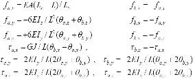
Where θ is the included angle that is defined by the orientation of the beam end and the axial direction of the beam. Its geometric definition is shown in Fig. 2.

For a rigid joint its corresponding orientations of the beam-ends, orientations of the beam-ends connected to that joint, maintain their relative difference in the transient phase. For a straight joint, the two corresponding orientations of the beam-ends coincide with each other throughout the process. Therefore, by assigning orientations as in Fig. 3a, we can assign the pre-stress of an initially straight joint. The assignment of an initially angled joint is shown in Fig. 3b.

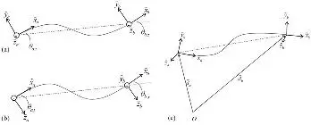
Fig. 2 (a) Definitions of included angles, θa,z and θb,z ; (b) Definitions of included angles, θa,y and θb,y ; and (c) Definitions of the beam axial direction, .

For a rigid joint its corresponding orientations of the beam-ends, orientations of the beam-ends connected to that joint, maintain their relative difference in the transient phase. For a straight joint, the two corresponding orientations of the beam-ends coincide with each other throughout the process. Therefore, by assigning orientations as in Fig. 3a, we can assign the pre-stress of an initially straight joint. The assignment of an initially angled joint is shown in Fig. 3b.

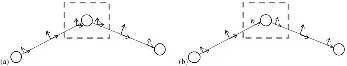
Fig. 3 (a) In the area enclosed by the dashed line, the orientations of the consecutive beam ends are equivalent. This builds up the pre-stress of moments of an initially straight joint; (b) In the area enclosed by the dashed line, the orientations of the two consecutive beam ends are the same as its own beam orientation. Hence no pre-stress of moments and torsion is built.

In our scheme, the profile stiffness can be used as an active factor in the form-finding process. The real stiffness - a profile stiffness of a practical profile that can be used in the bearing structure - is useful to explore the structural behaviour of elastic grids under geometric constraints. Besides, if the grid lengths are pre-determined, the real stiffness is helpful to solve a grid pattern in accordance with these pre-determined grid lengths.

If minimising the bending strain energy is a more critical issue than maintaining grid lengths, the fictitious stiffness - a profile stiffness that is designed on purpose and is only used in the form-finding stage - is used, which is defined by multiplying the bending and torsional stiffness by a weighted factor lager than one and keeping the axial stiffness unchanged. The fictitious stiffness enables the grids to have a larger range of strained lengths, which is helpful to reduce curvatures of the bending elements. Besides, this character can be utilised to generate smoothly curved grid patterns with various grid lengths.