Rethinking Prototyping
Здесь есть возможность читать онлайн «Rethinking Prototyping» — ознакомительный отрывок электронной книги совершенно бесплатно, а после прочтения отрывка купить полную версию. В некоторых случаях можно слушать аудио, скачать через торрент в формате fb2 и присутствует краткое содержание. Жанр: unrecognised, на английском языке. Описание произведения, (предисловие) а так же отзывы посетителей доступны на портале библиотеки ЛибКат.
- Название:Rethinking Prototyping
- Автор:
- Жанр:
- Год:неизвестен
- ISBN:нет данных
- Рейтинг книги:3 / 5. Голосов: 1
-
Избранное:Добавить в избранное
- Отзывы:
-
Ваша оценка:
Rethinking Prototyping: краткое содержание, описание и аннотация
Предлагаем к чтению аннотацию, описание, краткое содержание или предисловие (зависит от того, что написал сам автор книги «Rethinking Prototyping»). Если вы не нашли необходимую информацию о книге — напишите в комментариях, мы постараемся отыскать её.
The Design Modelling Symposium Berlin 2013 would like to challenge the participants to reflect on the possibility of computational systems that bridge design phase and occupancy of buildings. This rethinking of the designed artifact beyond its physical has had profound effects on other industries already. How does it affect architecture and engineering?
At the scale of engineering and building systems new perspectives may open up by engaging built form as a continuous prototype, which can track and respond during use and serve as a real world implementation of its design model. This has been tried many times from intelligent façades to smart homes and networked grids but much of it was only technology driven and not approached from a more holistic design perspective.
Rethinking Prototyping — читать онлайн ознакомительный отрывок
Ниже представлен текст книги, разбитый по страницам. Система сохранения места последней прочитанной страницы, позволяет с удобством читать онлайн бесплатно книгу «Rethinking Prototyping», без необходимости каждый раз заново искать на чём Вы остановились. Поставьте закладку, и сможете в любой момент перейти на страницу, на которой закончили чтение.
Интервал:
Закладка:
3 Geometric Constraint
In contrast with the implicit integration method the explicit method does not require a global stiffness matrix. The motion update is treated locally for each node. The nodal motion is only affected by the physical quantities around the node. As a result, DR is an ideal method to deal with local perturbations that are caused by physical contacts or geometric constraints, because the local instability will not cause the entire system to crash. The geometric constraint discussed in this paper is a curve or surface defined by the non-uniform rational basis spline (NURBS). If a structural node is constrained, its movement will be restricted within the constraint domain. The static state derived in this manner is a state that exhibits the lowest strain energy while satisfying all geometric constraints, which is crucial for combining material aspects with geometric design requirements.
3.1 Projection Method
By counting only tangential nodal residuals, a smooth tangential movement on the constraint surface/curve is achieved. The slight deviation caused by the tangential movement is adjusted by projecting the constrained node to the constraint at the end of each time step.
3.2 Constraint Force Method
We can also manipulate the form by applying constraint forces. A nodal constraint force may be defined by a vector which points toward the closest point on the geometric constraint and is proportional to the distance between the node and the point.
The magnitude of the constraint force is used to control the fitness of the obtained form to the target geometry. Smaller constraint forces result in a form that exhibits less strain energy but with the price of a larger deviation from the target geometry. An agreeable result may be attained by tuning the magnitude of the constraint forces.
4 Examples
Four examples are presented in this section. The first example shows a beam that is relaxed from a strained geometry. The second example demonstrates the form-finding process of a single-layer grid shell. The third example and the fourth example show the form-finding processes of double-layer grid structures.
4.1 Relaxed Beam
This example is used to verify the pre-stress assignment as proposed in Sec. 2. If the pre-stress is correct, the strained curved beam will resume a straight line as in Fig. 4. The diameter of the barrel and the length of the barrel are 20m and 40m respectively. The initial geometry of the bended beam is defined as a helix on the barrel. The beam is composed of 36 elements with a square profile that has a side length of 5cm. Each element has a length of 141cm. The elasticity and shear modulus are defined by E=107KN/m 2 and G=E/2 , respectively.
Once the beam is released, the motion is triggered by the residuals and the system is eventually damped to a static state. The computation terminates once the residual of each node is less than 10-4KN. The variation in strain energy throughout the process is shown in Fig. 5.
4.2. Weald and Downland Gridshell
The Downland Gridshell , which is charcaterised for its unique triple-bulb geometry, is our first form-finding example. The task is to find a single-layer grid pattern that complies with the material aspects and satisfies the geometric constraints.

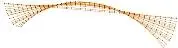
Fig. 4 (a) Pre-stressed beam on a barrel surface; (b) Beam relaxed from a strained geometry
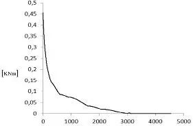
Fig. 5 Strain energy versus time step
The grid, which is composed of 102 initially straight planks, has a uniform square profile and a width of 5cm (Fig.6). Each beam element has an unstrained length of 1m. The connections between the crossing rods are revolute joints, which enable free rotation along the local z-direction. The elasticity and shear modulus of the material are defined as E=10 7 KN/m 2 and G=E/2 , respectively.
Two geometrical constraints are given. First, the grid nodes on the two longer edges must stay on the curved boundaries. Second, the remaining grid nodes must remain on the triple-bulb surface.
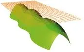
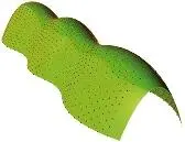
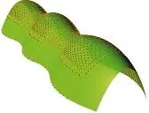

Fig. 6 (a) Initial grid and geometric constraints; (b) Transient state; (c) Equilibrium state under constraint; (d) Bearing structure after constraints are removed and bracing and bearing conditions are added; the enlarged part shows the nodal orientations.
4.3. Effect of the Weighted Stiffness (Irregular Gridshell)
In this example, we apply the weighted stiffness in the form-finding stage to the above grid structure to see its effect on the grid patterns: A factor of 10E4 is applied to the bending and torsional stiffness to enable the beam element to have a larger range of the strained length. This fictitious stiffness setting is only used in the form-finding stage. Once the form is found, the material stiffness is recovered and the strained lengths of the found form are taken as the new unstrained grid lengths.
The comparison of the strain energy between the two forms, which are found with the real stiffness setting and the fictitious stiffness setting, is showed in Tab. 2, and the comparison of their geometries is showed in Fig. 7. The in-plane bending strain energy of the irregular grid shell is largely reduced, which is only 25% of the in-plane bending strain energy of the regular gridshell.
| Table 2: Comparisons of the grid length and the strain energy between the regular grid and the irregular grid | |||||||
| max. length[m] | min. length[m] | strain energy [kNm] | axial strain energy [kNm] | torsional strain energy [kNm] | out-of-plane bending strain energy [kNm] | in-plane be ding strain energy [kNm] | |
| regular grid irregular grid | 1.0003 1.0602 | 0.9996 0.9308 | 9.5E+01 6.7E+01 | 5.2E-01 3.2E-03 | 2.5E+01 2.6E+01 | 3.6E+01 3.3E+01 | 3.2E+01 8.2E+00 |
4.4 2D Hybgrid
Hybgrid , which was proposed by Truco and Felipe [8], is an innovative double-layer structural type that is composed of uniform flexible chord members and can generate various geometries by controlling the strut lengths between the chords (Fig. 8). Currently, the only available form-finding for Hybgrid is based on physical models. Thus, the testing of our method constitutes a significant benchmark.
Читать дальшеИнтервал:
Закладка:
Похожие книги на «Rethinking Prototyping»
Представляем Вашему вниманию похожие книги на «Rethinking Prototyping» списком для выбора. Мы отобрали схожую по названию и смыслу литературу в надежде предоставить читателям больше вариантов отыскать новые, интересные, ещё непрочитанные произведения.

Обсуждение, отзывы о книге «Rethinking Prototyping» и просто собственные мнения читателей. Оставьте ваши комментарии, напишите, что Вы думаете о произведении, его смысле или главных героях. Укажите что конкретно понравилось, а что нет, и почему Вы так считаете.