Richard J. Rossi - Applied Biostatistics for the Health Sciences

Examples of the binomial distribution are given in Figure 2.24. Note that a binomial distribution will have a longer tail to the right when p < 0.5, a longer tail to the left when p > 0.5, and is symmetric when p = 0.5.

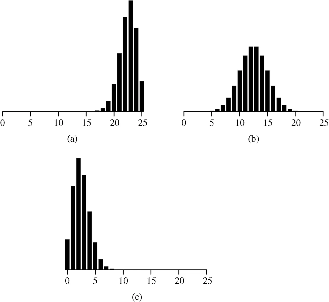
Figure 2.24 Three binomial distributions: (a) n=25,p=0.1; (b) n=25,p=0.5; (c) n=25,p=0.9.

Because the computations for the probabilities associated with a binomial random variable are tedious, it is best to use a statistical computing package such as MINITAB for computing binomial probabilities.

Example 2.31

Hair loss is a common side effect of chemotherapy. Suppose that there is an 80% chance that an individual will lose their hair during or after receiving chemotherapy. Let X be the number of individuals who retain their hair during or after receiving chemotherapy. If 10 individuals are selected at random, use the MINITAB output given in Table 2.10to determine

Table 2.10 The Binomial Distribution for n= 10 Trials and p = 0.20

1 the probability that exactly seven will retain their hair (i.e., X = 7),

2 the probability that between four and eight (inclusive) will retain their hair (i.e., 4≤X≤8),

3 the probability that at most three will retain their hair (i.e., X≤3),

4 the probability that at least six will retain their hair (i.e., X≥6),

5 the most likely number of patients to retain their hair (i.e., the mode).

Solutions

Based on the MINITAB output in Table 2.10, the probability that

1 exactly seven will retain their hair (i.e., X = 7) is

2 between four and eight (inclusive) will retain their hair (i.e., 4≤X≤8) is

3 at most three will retain their hair (i.e., X≤3) is

4 at least six will retain their hair (i.e., X≥6) is

5 the most likely number of patients to retain their hair is X = 2.

The mean of a binomial random variable based on n trials and probability of success p is μ=np and the standard deviation is σ=n⋅p⋅(1−p). The mean of a binomial is the expected number of successes in n trials, and the values of a binomial random variable are concentrated near its mean. The standard deviation measures the spread about the mean and is largest when p = 0.5; as p moves away from 0.5 toward 0 or 1, the variability of a binomial random variable decreases. Furthermore, when np and n(1−p) are both greater than 5, the apply and

roughly 68% of the binomial distribution lies between the values closest to the np−n⋅p⋅(1−p) and np+n⋅p⋅(1−p),

roughly 95% of the binomial distribution lies between the values closest to np−2n⋅p⋅(1−p) and np+2n⋅p⋅(1−p),

roughly 99% of the binomial distribution lies between the values closest to np−3n⋅p⋅(1−p) and np+3n⋅p⋅(1−p).

Example 2.32

Suppose the relapse rate within 3 months of treatment at a drug rehabilitation clinic is known to be 40%. If the clinic has 25 patients, then the mean number of patients to relapse within 3 months is μ=25⋅0.40=10 and the standard deviation is σ=25⋅0.40⋅(1−0.40)=2.45. Now, since np=25(0.4)=10 and n(1−p)=25(0.6)=15, by applying the Empirical Rules roughly 95% of the time between 5 and 15 patients will relapse within 3 months of treatment. Using MINITAB, the actual percentage of a binomial distribution with n = 25 and p = 0.40 falling between 5 and 15 is 98%.

An important restriction in the setting for a binomial random variable is that the probability of success remains constant over the n trials. In many biomedical studies, the probability of success will be different for each individual in the experiment because the individuals are different. For example, in a study of the survival of patients having suffered heart attacks, the probability of survival will be influenced by many factors including severity of heart attack, delay in treatment, age, and ability to change diet and lifestyle following a heart attack. Because each individual is different, the probability of survival is not going to be constant over the n individuals in the study, and hence, the binomial probability model does not apply.

The choice of a probability model for continuous variables is generally based on historical data rather than a particular set of conditions. Just as there are many discrete probability models, there are also many different probability models that can be used to model the distribution of a continuous variable. The most commonly used continuous probability model in statistics is the normal probability model .

The normal probability model is often used to model distributions that are expected to be unimodal and symmetric, and the normal probability model forms the foundation for many of the classical statistical methods used in biostatistics. Moreover, the distribution of many natural phenomena can be modeled very well with the normal distribution. For example, the weights, heights, and IQs of adults are often modeled with normal distributions.

Several properties of a normal distribution are listed below.

A normal distribution

is a bell- or mound-shaped distribution.

is completely characterized by its mean and standard deviation. The mean determines the center of the distribution and the standard deviation determines the spread about the mean.

has probabilities and percentiles that are determined by the mean and standard deviation.

is symmetric about the mean.

has mean, median, and mode that are equal (i.e., μ=μ~=M).

has probability density function given by

Example 2.33

The intelligence quotient (IQ) is based on a test of aptitude and is often used as a measure of an individual’s intelligence. The distribution of IQ scores is approximately normally distributed with mean 100 and standard deviation 15. The normal probability model for IQ scores is given in Figure 2.25.

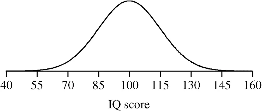
Figure 2.25 The approximate distribution of IQ scores with µ = 100 and σ = 15.

The standard normal, which will be denoted by Z , is a normal distribution having mean 0 and standard deviation 1. The standard normal is used as the reference distribution from which the probabilities and percentiles associated with any normal distribution will be determined. The cumulative probabilities for a standard normal are given in Tables A.1 and A.2; because 99.95% of the standard normal distribution lies between the values −3.49 and 3.49, the standard normal values are only tabulated for z values between −3.49 and 3.49. Thus, when the value of a standard normal, say z , is between −3.49 and 3.49, the tabled value for z represents the cumulative probability of z , which is P(Z≤z) and will be denoted by Φ(z). For values of z below −3.50, Φ(z) will be taken to be 0 and for values of z above 3.50, Φ(z) will be taken to be 1. Tables A.1 and A.2 can be used to compute all of the probabilities associated with a standard normal.