Richard J. Rossi - Applied Biostatistics for the Health Sciences
Здесь есть возможность читать онлайн «Richard J. Rossi - Applied Biostatistics for the Health Sciences» — ознакомительный отрывок электронной книги совершенно бесплатно, а после прочтения отрывка купить полную версию. В некоторых случаях можно слушать аудио, скачать через торрент в формате fb2 и присутствует краткое содержание. Жанр: unrecognised, на английском языке. Описание произведения, (предисловие) а так же отзывы посетителей доступны на портале библиотеки ЛибКат.

- Название:Applied Biostatistics for the Health Sciences
- Автор:
- Жанр:
- Год:неизвестен
- ISBN:нет данных
- Рейтинг книги:3 / 5. Голосов: 1
-
Избранное:Добавить в избранное
- Отзывы:
-
Ваша оценка:
Applied Biostatistics for the Health Sciences: краткое содержание, описание и аннотация
Предлагаем к чтению аннотацию, описание, краткое содержание или предисловие (зависит от того, что написал сам автор книги «Applied Biostatistics for the Health Sciences»). Если вы не нашли необходимую информацию о книге — напишите в комментариях, мы постараемся отыскать её.
APPLIED BIOSTATISTICS FOR THE HEALTH SCIENCES Applied Biostatistics for the Health Sciences
Applied Biostatistics for the Health Sciences
Applied Biostatistics for the Health Sciences — читать онлайн ознакомительный отрывок
Ниже представлен текст книги, разбитый по страницам. Система сохранения места последней прочитанной страницы, позволяет с удобством читать онлайн бесплатно книгу «Applied Biostatistics for the Health Sciences», без необходимости каждый раз заново искать на чём Вы остановились. Поставьте закладку, и сможете в любой момент перейти на страницу, на которой закончили чтение.
Интервал:
Закладка:
The values of z are referenced in Tables A.1 and A.2 by writing z=a.bc as z=a.b+0.0c. To locate a value of z in Table A.1 and A.2, first look up the value a.b in the left-most column of the table and then locate 0.0 c in the first row of the table. The value cross-referenced by a.b and 0.c in Tables A.1 and A.2 is Φ(z)=P(Z≤z). The rules for computing the probabilities for a standard normal are given below.
COMPUTING STANDARD NORMAL PROBABILITIES
1 For values of z between −3.49 and 3.49, the probability that Z≤z is read directly from the table. That is,
2 For z≤−3.50 the probability that Z≤z is 0, and for z≥3.50 the probability that Z≤z is 1.
3 For values of z between −3.49 and 3.49, the probability that Z≥z is
4 For values of z between −3.49 and 3.49, the probability that a≤Z≤b is
Example 2.34
To determine the probability that a standard normal random variable is less than 1.65, which is the area shown in Figure 2.26, look up 1.6 in the left-most column of Table A.2 and 0.05 in the top row of this table, which yields P(Z≤1.65)=0.9505.
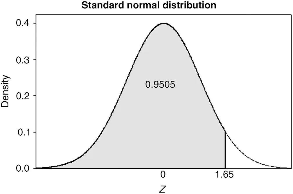
Figure 2.26 P(Z≤1.65).
Example 2.35
Determine the probability that a standard normal random variable lies between −1.35 and 1.51 (see Figure 2.27).
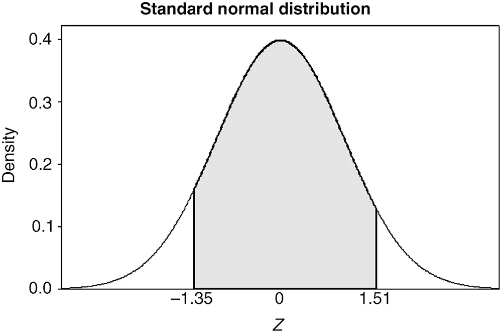
Figure 2.27 P(−1.35≤Z≤1.51).
SolutionsFirst, look up the cumulative probabilities for both −1.35 and 1.51 in Tables A.1 and A.2. The probability that Z≤−1.35 and the probability that Z≤1.51 are shown in Figure 2.28.
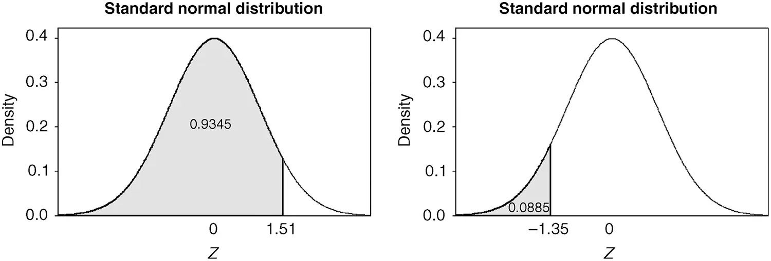
Figure 2.28 The areas representing P(Z≤1.51) and P(Z≤−1.35).
Subtracting these probabilities yields P(−1.35≤Z≤1.51), and thus,

Example 2.36
Using the standard normal tables given in Tables A.1 and A.2, determine the following probabilities for a standard normal distribution:
1 P(Z≤−2.28)
2 P(Z≤3.08)
3 P(−1.21≤Z≤2.28)
4 P(1.21≤Z≤6.28)
5 P(−4.21≤Z≤0.84)
SolutionsUsing the normal table in the appendix
1 P(Z≤−2.28)=Φ(−2.28)=0.0113
2 P(Z≥3.08)=1−Φ(3.08)=1−0.9990=0.0010
3 P(−1.21≤Z≤2.28)=Φ(1.81)−Φ(−1.21)=0.9887−0.1131=0.8756
4 P(0.67≤Z≤6.28)=Φ(6.28)−Φ(0.67)=1−0.7486=0.2514
5 P(−4.21≤Z≤0.84)=Φ(0.84)−0=0.7995
The p th percentile of the standard normal can be found by looking up the cumulative probability p100 inside of the standard normal tables given in Appendix A and then working backward to find the value of Z . Unfortunately, in some cases the value of p100 will not be listed inside the table, and in this case, the value closest to p100 inside of the table should be used for finding the approximate value of the p th percentile.
Example 2.37
Determine the 90th percentile of a standard normal distribution.
SolutionsTo find the 90th percentile, the first step is to find 90100=0.90, or the value closest to 0.90, in the cumulative standard normal table. The row of the standard normal table containing the value 0.90 is given in Table 2.11. Since 0.8997 is the value closest to 0.90 that occurs in the row labeled 1.2 and the column labeled 0.08, the 90th percentile of a standard normal distribution is roughly z=1.2+0.08=1.28.
Table 2.11 An Excerpted Section of the Cumulative Normal Table
| Φ(z)=P(Z≤z) | ||||||||||
|---|---|---|---|---|---|---|---|---|---|---|
| z | 0.00 | 0.01 | 0.02 | 0.03 | 0.04 | 0.05 | 0.06 | 0.07 | 0.08 | 0.09 |
| ⋮ | ||||||||||
| 1.2 | 0.8849 | 0.8869 | 0.8888 | 0.8907 | 0.8925 | 0.8944 | 0.8962 | 0.8980 | 0.8997 | 0.9015 |
| ⋮ |
The most commonly used percentiles of the standard normal are given in Table 2.12, and a more complete list of the percentiles of the standard normal distribution is given in Table A3. Note that for p < 50 the percentiles of a standard normal are negative, for p = 50 the 50th percentile is the median, and for p > 50 the percentiles of a standard normal are positive.
Table 2.12 Selected Percentiles of a Standard Normal Distribution
| p | 1 | 5 | 10 | 20 | 25 | 50 |
| p th percentile | −2.33 | −1.645 | −1.28 | −0.84 | −0.67 | 0.00 |
| p | 75 | 80 | 90 | 95 | 99 | 99.9 |
| p th percentile | 0.67 | 0.84 | 1.28 | 1.645 | 2.33 | 3.09 |
When X is a normal distribution with μ≠0 or σ≠1, the distribution of X is called a non-standard normal distribution . The standard normal distribution is the reference distribution for all normal distributions because all of the probabilities and percentiles for a non-standard normal can be determined from the standard normal distribution. In particular, the following relationships between a non-standard normal with mean µ and standard deviation σ and the standard normal can be used to convert a non-standard normal value to a Z -value and vice versa.
THE RELATIONSHIPS BETWEEN A STANDARD NORMAL AND A NON-STANDARD NORMAL
1 If X is a non-standard normal with mean µ and standard deviation σ, then Z=(X−μ)/σ.
2 If Z is a standard normal, then X=σ⋅Z+μ is a non-standard normal with mean µ and standard deviation σ.
Note that the value of a non-standard normal X can be converted into a Z -value and vice versa. The first equation shows that centering and scaling the values of X converts them to Z -values, and the second equation shows how to convert a Z -value into an X -value. The relationship between a standard normal and a non-standard normal is shown in Figure 2.29.
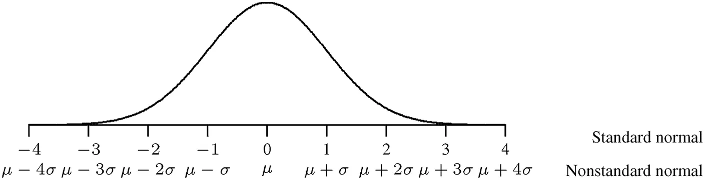
Figure 2.29 The correspondence between the values of a standard normal and a non-standard normal.
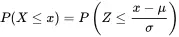
To determine the cumulative probability for the value of a non-standard normal, say x , convert the value of x to its corresponding z value using z=z−μ/σ; then determine the cumulative probability for this z value. That is,
To compute probabilities other than a cumulative probability for a non-standard normal, note that the probability of being in any region can also be computed from the cumulative probabilities associated with the standard normal. The rules for computing the probabilities associated with a non-standard normal are given below.
Читать дальшеИнтервал:
Закладка:
Похожие книги на «Applied Biostatistics for the Health Sciences»
Представляем Вашему вниманию похожие книги на «Applied Biostatistics for the Health Sciences» списком для выбора. Мы отобрали схожую по названию и смыслу литературу в надежде предоставить читателям больше вариантов отыскать новые, интересные, ещё непрочитанные произведения.


Обсуждение, отзывы о книге «Applied Biostatistics for the Health Sciences» и просто собственные мнения читателей. Оставьте ваши комментарии, напишите, что Вы думаете о произведении, его смысле или главных героях. Укажите что конкретно понравилось, а что нет, и почему Вы так считаете.