Philip Hofmann - Solid State Physics

In more complex solids, several bonding types can coexist. For instance, the diamond structure of Figure 1.7is also found for materials that mix group III and group V elements, such as GaAs, or group II and group VI elements, such as InP. In these, the different atoms occupy alternating sites but still adopt the bonding arrangement. This is accompanied by an electron transfer from the higher‐group atom to the lower‐group atom, resulting in a bonding situation with both covalent and ionic contributions.

We now return to the Schrödinger equation for the full Hamiltonian from Eq. (2.3). This has to be solved by a wave function containing the coordinates and of two electrons (we still keep the positions of the nuclei fixed). This makes the problem much harder and we can only begin to imagine the difficulty of finding a wave function describing all the electrons in a solid! Fortunately, even in a solid, most cases can be described quite well by considering one electron moving in the potential of the ions and some averaged potential arising from the other electrons. In this book, there are only two cases where this simple description will fail: magnetism and superconductivity. The following discussion will mainly be useful for the treatment of magnetism in Chapter 8. Understanding these details is not crucial at this point, and you could decide to jump to Section 2.4and return here later.

Solving the Schrödinger equation for the Hamiltonian from Eq. (2.3) would be greatly simplified if we could somehow “switch off” the electrostatic interaction between the two electrons, because then the Hamiltonian could be written as the sum of two parts, one for each electron. Indeed, the Hamiltonian in Eq. (2.3) could essentially be the sum of two Hamiltonians similar to the one in Eq. (2.4), one for each electron (but with the term appearing only once). If a Hamiltonian containing two electronic coordinates could be separated into a sum of two Hamiltonians that contain only one electronic coordinate each, the corresponding Schrödinger equation could be solved by a product of the two wave functions that are solutions to the two individual Hamiltonians. We could therefore start an attempt to solve Eq. (2.3) based on what we have already learned for the ion. However, we will start from an even simpler point of view: Without any interaction between the electrons, and for a large distance , the electron near nucleus A will not feel the potential of nucleus B and vice versa. In this case, Eq. (2.3) would simply turn into the sum of the Hamiltonians for two hydrogen atoms and we could approximate the two‐electron wave function by 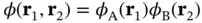, with and being the wave functions for atomic hydrogen.

However, this simple approach is physically incorrect because such a wave function does not obey the Pauli principle. Since the electrons are fermions, the total wave function must be antisymmetric with respect to particle exchange, and the simple product wave function does not meet this requirement. The total wave function consists of a spatial part and a spin part, and thus there are two possibilities for forming an antisymmetric wave function – we can either combine a symmetric spatial part with an antisymmetric spin part or vice versa. The spatial part of the wave function can be constructed in two ways,

(2.9)

(2.10)

The plus sign in Eq. (2.9) returns a symmetric spatial wave function, which we can combine with an antisymmetric spin wave function with the total spin equal to zero (the so‐called singlet state); the minus in Eq. (2.10) results in an antisymmetric spatial wave function to be combined with a symmetric spin wave function with the total spin equal to 1 (the so‐called triplet state).

The antisymmetric wave function in Eq. (2.10)vanishes for – that is, the two electrons cannot be at the same location simultaneously. This leads to a depletion of the electron density between the nuclei and hence to an antibonding state. For the symmetric case, on the other hand, the electrons have opposite spins and can be at the same place, which leads to a charge accumulation between the nuclei and hence to a bonding state (see Figure 2.4).

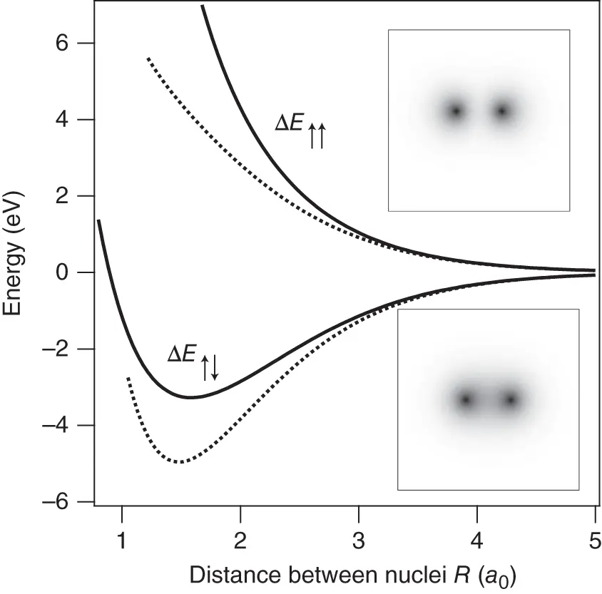
Figure 2.4 The energy changes and for the formation of a hydrogen molecule. The dashed lines represent the approximation for long distances. The two insets show grayscale images of the corresponding electron probability density.

An approximate way to calculate the eigenvalues of Eq. (2.3) was suggested by W. Heitler and F. London in 1927. Their approach was to use the known single‐particle 1s wave functions for atomic hydrogen for and to form a two‐electron wave function , in the form of either Eq. (2.9) or Eq. (2.10). These wave functions might not be entirely correct because the atomic wave functions will certainly be modified by the presence of the other atom. However, even if they are only approximately correct, we can obtain the molecular energy levels as

(2.11)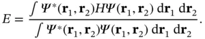

According to the variational principle in quantum mechanics, the resulting energy will always be higher than the correct ground‐state energy, but it will approach it for a good choice of the trial wave functions.