Philip Hofmann - Solid State Physics

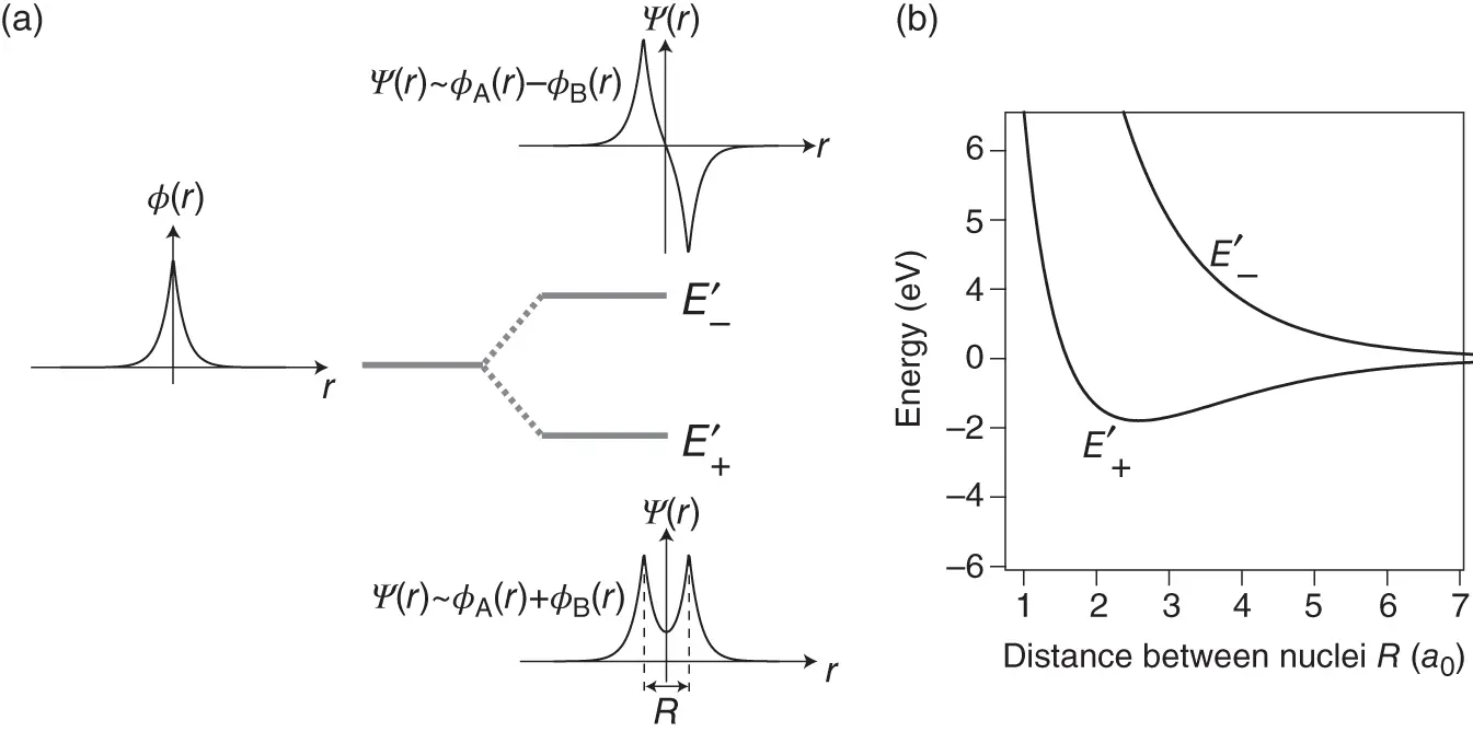
Figure 2.2 (a) Formation of bonding and antibonding energy levels in the ion. The electronic energy level of an isolated H atom splits into the levels according to Eq. (2.8). The radial wave function of an isolated H atom is shown at the left, and the bonding and antibonding wave functions along the molecular axis of the ion are shown at the right (for proper normalization see Problem 3). (b) Bonding and antibonding energy levels as a function of internuclear distance . Zero energy corresponds to the ground state energy of a free hydrogen atom.

Figure 2.2b shows how the energy levels vary as a function of the distance between the nuclei. The antibonding energy increases monotonically as the nuclei approach each other, but the bonding energy has a minimum of eV at approximately twice the Bohr radius . With the single electron placed into the bonding state , the total energy gain resulting from formation of the covalent bond is thus 1.77 eV. It is tempting to extend this model to the two electrons in the molecule by placing the second electron in the same energy level. This electron would then also lower its energy by 1.77 eV, amounting to a total energy gain of 3.54 eV for the formation of the hydrogen molecule. Handling the additional electron in this way is too simplistic, as we shall see below, but the energy gain thus computed is at least similar to the experimental value of eV. It is also clear that no additional electrons can be placed in the energy level, as this would violate the Pauli principle. A third electron would need to occupy the level, destabilizing the molecule as compared to with two electrons. In covalently bonded solids, each atom forms bonds to several neighbors and the total energy gain per atom can be higher than for . In silicon, for example, the energy gain per atom (or cohesive energy) is 4.6 eV.

Apart from a high cohesive energy, a characteristic feature of covalent bonding is the directional nature of the bonds. The preference for certain bond directions governs the crystal structures of covalently bonded solids, and these are more complex than the close‐packed structures typically encountered in metals. The treatment of the molecular ion has demonstrated the idea of constructing bonding and antibonding molecular orbitals from a linear combination of atomic orbitals, but since we combined two isotropic 1s orbitals in this case, the directional character of covalent bonding did not emerge.

Figure 2.3demonstrates the consequences of using directional orbitals, such as p orbitals, for the formation of wave functions in molecules or solids. Figure 2.3a represents the case that we have just treated. Two s orbitals are combined to produce a bonding and an antibonding orbital by being added either in phase or out of phase (as indicated by the shading and the sign on the wave function). Due to the symmetry of the s orbital, the bond direction is not important. Combining an s orbital with a p orbital along the interatomic axis works in the same way (see Figure 2.3b). The p orbital is strongly anisotropic, but still the direction between the atoms does not matter in this case, because we define the intermolecular axis as the axis and then use the orbital aligned in this direction to form bonding and antibonding states. However, in this arrangement, no bonding interactions are possible between the s orbital of the left atom and the and orbitals of the right atom. This is illustrated in Figure 2.3c. No matter what linear combination coefficients we use, the overlap of the wave functions contains equal and mutually canceling bonding and antibonding contributions. This dilemma is the source of the directional preference in covalent bonding. In order to achieve the highest energy gain, it is often favorable to use linear combinations of the orbitals in one atom before combining them with other atoms. Examples for this are the and hybrid orbitals found in carbon‐based solids such as diamond or graphite, which directly explain the preferred bonding directions shown in Figure 1.7. The orbitals in graphene are also shown in Figure 6.15a. All these orbitals are highly directional.

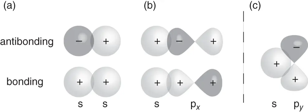
Figure 2.3 Linear combination of orbitals on neighboring atoms. (a) Two s orbitals as in the molecular ion. (b) An s orbital and a orbital (the choice of the direction is arbitrary). (c) An s orbital with a or orbital. Due to symmetry, the total overlap is zero and no bonding or antibonding orbitals can be formed.