Enrico Zio - Reliability Analysis, Safety Assessment and Optimization

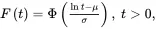
where σ>0 is the shape parameter and μ>0 is the scale parameter of the distribution. Note that the lognormal variable is developed from the normal distribution. The random variable X=lnT is a normal random variable with parameters μ and σ. The cdf of the lognormal distribution is

(1.39)

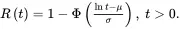
where Φ(x) is the cdf of a standard normal random variable. If T denotes the failure time of an item with lognormal distribution, the reliability function of T will be

(1.40)

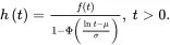
The hazard rate function is

(1.41)

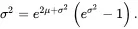
The mean, μ, and variance, σ2, are

(1.42)

Example 1.3

The random variable of the time to failure of an item, T, follows the following pdf:

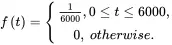
where t is in days and t≥0.

1 What is the probability of failure of the item in the first 100 days?

2 Find the MTTF of the item.

Solution

1 The cdf of the random variable isThe probability of failure in the first 100 days is

2 The MTTF of the item is

Different from the traditional reliability assessment approach, the Physics-of-Failure (P-o-F) represents an approach to reliability assessment based on modeling and simulation of the physical processes leading to the occurrence of failures in an item [2]. The P-o-F approach begins within the first stages of the design of the item. A model is constructed based on the customer’s requirements, service environment, and stress analysis [1]. Once the models are established, a reliability assessment can be conducted on the item.

Paris’ law is a crack growth equation that gives the rate of growth of a fatigue crack [3]. The stress intensity factor K characterizes the load around a crack tip and the rate of crack growth is experimentally shown to be a function of the range of the stress intensity ΔK experienced in a loading cycle (shown in Figure 1.7). The Paris’ equation describing this is

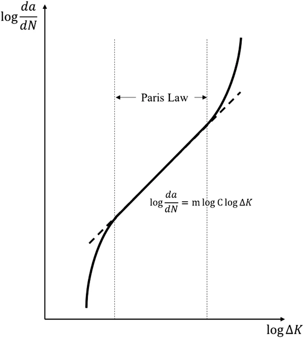
Figure 1.7 Illustration of Paris Law.

(1.43)

where a is the crack length and dadN is the fatigue crack growth for a load cycle N. The material coefficients C and m are obtained experimentally and their values depend on environment, temperature, and stress ratio. The stress intensity factor range has been found to correlate with the rate of crack growth in a variety of different conditions, which is the difference between the maximum and minimum stress intensity factors in a load cycle, defined as

(1.44)

The Archard’s wear equation is a simple model used to describe sliding wear, which is based on the theory of asperity contact [4]. The volume of the removed debris due to wear is proportional to the work done by friction forces. The Archard’s wear equation is given by

(1.45)

where Q is the total volume of the wear debris produced, K is a dimensionless constant, W is the total normal load, L is the sliding distance, and H is the hardness of the softest contacting surfaces. It is noted that WL is proportional to the friction forces. K is obtained from experimental results and it depends on several parameters, among which are surface quality, chemical affinity between the material of two surfaces, surface hardness process, etc.

The methods to model and estimate the reliability of a single component were introduced in Section 1.2. Compared with the single component case, the system reliability modeling and assessment is more complicated. The term ‘system’ is used to indicate a collection of components working together to perform a specific function. The reliability of a system depends not only on the reliability of each component but also on the structure of the system, the interdependence of its components, and the role of each component within the system, etc. To compute the reliability of the system, it is essential to construct the model of the system, representing the above characteristics.

The conventional approaches typically assume that the components and the system have two states: perfect working and complete failure [5]. Below, we introduce the reliability models of a binary state system with specific structures. Details about the multi-state system can be found in Chapter 3.

In a series system, all components must operate successfully for the system to function or operate successfully. It implies that the failure of any component will cause the entire system to fail. The reliability block diagram of a series system is shown in Figure 1.8.

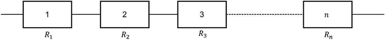
Figure 1.8 Reliability block diagram of a series system.

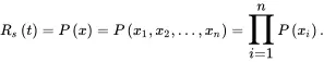
Let Ri(t) be the reliability of the ith component, i=1,2,…,n,, and Rs(t) be the reliability of the system. Let xi be the event that the ith component is operational and let x be the event that indicates system is operational. The reliability of the series system can be calculated by

(1.46)

Assume all the components in the series system are independent; if so, the reliability of the system can be expressed as

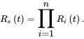(1.47)

Considering that the component reliability is a number between 0 and 1, we have the following relationship

(1.48)