Enrico Zio - Reliability Analysis, Safety Assessment and Optimization
Здесь есть возможность читать онлайн «Enrico Zio - Reliability Analysis, Safety Assessment and Optimization» — ознакомительный отрывок электронной книги совершенно бесплатно, а после прочтения отрывка купить полную версию. В некоторых случаях можно слушать аудио, скачать через торрент в формате fb2 и присутствует краткое содержание. Жанр: unrecognised, на английском языке. Описание произведения, (предисловие) а так же отзывы посетителей доступны на портале библиотеки ЛибКат.
- Название:Reliability Analysis, Safety Assessment and Optimization
- Автор:
- Жанр:
- Год:неизвестен
- ISBN:нет данных
- Рейтинг книги:3 / 5. Голосов: 1
-
Избранное:Добавить в избранное
- Отзывы:
-
Ваша оценка:
Reliability Analysis, Safety Assessment and Optimization: краткое содержание, описание и аннотация
Предлагаем к чтению аннотацию, описание, краткое содержание или предисловие (зависит от того, что написал сам автор книги «Reliability Analysis, Safety Assessment and Optimization»). Если вы не нашли необходимую информацию о книге — напишите в комментариях, мы постараемся отыскать её.
Reliability Analysis, Safety Assessment and Optimization — читать онлайн ознакомительный отрывок
Ниже представлен текст книги, разбитый по страницам. Система сохранения места последней прочитанной страницы, позволяет с удобством читать онлайн бесплатно книгу «Reliability Analysis, Safety Assessment and Optimization», без необходимости каждый раз заново искать на чём Вы остановились. Поставьте закладку, и сможете в любой момент перейти на страницу, на которой закончили чтение.
Интервал:
Закладка:
Notations
Notations: Part I
| t | time point |
| nf(t) | number of failed items |
| ns(t) | number of the survived items |
| n0 | sample size |
| T | random variable of the failure time |
| F(t) | cdf of failure time |
| f(t) | pdf of failure time |
| R(t) | reliability at time t |
| h(t) | hazard function at time t |
| H(t) | cumulative hazard function at time t |
| Q^(t) | estimate of the unreliability |
| R^(t) | estimate of the reliability |
| D(t) | component or system demand at time t |
| G(t) | performance function at time t |
| MTTF | mean time to failure |
| X | random variable |
| a | crack length |
| N | load cycle |
| Q | total volume of wear debris produced |
| Rs(t) | reliability of the system at time t |
| (⋅) | unreliability function of the system |
| C | cost |
| x | decision variable |
| g(x) | inequality constraints |
| h(x) | equality constraints |
| f(x) | criterion function |
| D=(V, A) | directed graph |
| d(⋅) | length of the shortest path |
Notations: Part II
| t | time point |
| S | state set |
| M | perfect state |
| x=(x1,…,xn) | component state vector |
| X=(X1,…,Xn) | state of all components |
| ϕ(⋅) | structure function of the system |
| gi | performance level of component i |
| λkji | transition rate of component i from state k to state j |
| Qkji(t) | kernel of the SMP analogous to λkji of the CTMC |
| Tni | time of the n-th transition of component i |
| Gni | performance of component i at the n-th transition |
| θjki(t) | probability that the process of component i starts from state j at time t |
| AφW(t) | availability with a minimum on performance of total φ at time t |
| ui(z) | universal generating function of component i |
| pij=Pr(Xi=j) | probability of component i being at state j |
| p(t) | state probability vector |
| λij(t) | transition rate from state i to state j at time t in Markov process |
| Λ | transition rate matrix |
| Π(⋅) | possibility function |
| N(⋅) | necessity function |
| Bel(⋅) | belief function |
| Pl(⋅) | plausibility function |
| F−1(⋅) | inverse function |
| E(⋅) | expectation equation |
| ⊗ | UGF composition operator |
| Π(⋅) | possibility function |
| N(⋅) | necessity function |
| Bel(⋅) | belief function |
| Pl(⋅) | plausibility function |
| F−1(⋅) | inverse function |
| E(⋅) | expectation equation |
| S(⋅) | system safety function |
| Risk(⋅) | system risk function |
| C(⋅) | cost function |
Notation: Part III
| ri | reliability of subsystem i |
| x=(x1,…,xn)T | decision variable vector |
| c=(c1,…,cn)T | coefficients of the objective function |
| b=(b1,…,bm)T | right-hand side values of the inequality constraints |
| z=(z1,z2,…,zM) | objective vector |
| xl*, l=1,2,…,L | set of optimal solutions |
| w=(w1,w2,…,wM) | weighting vector |
| x* | global optimal solution |
| R(⋅) | system reliability function |
| A(⋅) | system availability function |
| M(⋅) | system maintainability function |
| S(⋅) | system safety function |
| C(⋅) | cost function |
| Risk(⋅) | system risk function |
| RN | N-dimensional solution space |
| fi | i - th objective functions |
| gj | j-th equality constraints |
| hk | k-th inequality constraints |
| ω | random event |
| ξ=(q(ω)T, h(ω)T, T(ω)T) | second-stage problem parameters |
| W | recourse matrix |
| y(ω) | second-stage or corrective actions |
| Q(x) | expected recourse function |
| U | uncertainty set |
| u | uncertainty parameters |
| ζ | perturbation vector |
| Z | perturbation set |
| xu* | optimal solution under the uncertainty parameter u |
1 Reliability Assessment
Reliability is a critical attribute for the modern technological components and systems. Uncertainty exists on the failure occurrence of a component or system, and proper mathematical methods are developed and applied to quantify such uncertainty. The ultimate goal of reliability engineering is to quantitatively assess the probability of failure of the target component or system [1]. In general, reliability assessment can be carried out by both parametric or nonparametric techniques. This chapter offers a basic introduction to the related definitions, models and computation methods for reliability assessments.
1.1 Definitions of Reliability
According to the standard ISO 8402, reliability is the ability of an item to perform a required function, under given environmental and operational conditions and for a stated period of time without failure. The term “item” refers to either a component or a system. Under different circumstances, the definition of reliability can be interpreted in two different ways:
1.1.1 Probability of Survival
Reliability of an item can be defined as the complement to its probability of failure, which can be estimated statistically on the basis of the number of failed items in a sample. Suppose that the sample size of the item being tested or monitored is n0. All items in the sample are identical, and subjected to the same environmental and operational conditions. The number of failed items is n fand the number of the survived ones is n s, which satisfies
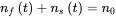 (1.1)
(1.1)
The percentage of the failed items in the tested sample is taken as an estimate of the unreliability,  ,
,
 (1.2)
(1.2)
Complementarily, the estimate of the reliability, R^(t), of the item is given by the percentage of survived components in the sample:
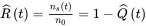 (1.3)
(1.3)
Интервал:
Закладка:
Похожие книги на «Reliability Analysis, Safety Assessment and Optimization»
Представляем Вашему вниманию похожие книги на «Reliability Analysis, Safety Assessment and Optimization» списком для выбора. Мы отобрали схожую по названию и смыслу литературу в надежде предоставить читателям больше вариантов отыскать новые, интересные, ещё непрочитанные произведения.


Обсуждение, отзывы о книге «Reliability Analysis, Safety Assessment and Optimization» и просто собственные мнения читателей. Оставьте ваши комментарии, напишите, что Вы думаете о произведении, его смысле или главных героях. Укажите что конкретно понравилось, а что нет, и почему Вы так считаете.