Enrico Zio - Reliability Analysis, Safety Assessment and Optimization
Здесь есть возможность читать онлайн «Enrico Zio - Reliability Analysis, Safety Assessment and Optimization» — ознакомительный отрывок электронной книги совершенно бесплатно, а после прочтения отрывка купить полную версию. В некоторых случаях можно слушать аудио, скачать через торрент в формате fb2 и присутствует краткое содержание. Жанр: unrecognised, на английском языке. Описание произведения, (предисловие) а так же отзывы посетителей доступны на портале библиотеки ЛибКат.
- Название:Reliability Analysis, Safety Assessment and Optimization
- Автор:
- Жанр:
- Год:неизвестен
- ISBN:нет данных
- Рейтинг книги:3 / 5. Голосов: 1
-
Избранное:Добавить в избранное
- Отзывы:
-
Ваша оценка:
Reliability Analysis, Safety Assessment and Optimization: краткое содержание, описание и аннотация
Предлагаем к чтению аннотацию, описание, краткое содержание или предисловие (зависит от того, что написал сам автор книги «Reliability Analysis, Safety Assessment and Optimization»). Если вы не нашли необходимую информацию о книге — напишите в комментариях, мы постараемся отыскать её.
Reliability Analysis, Safety Assessment and Optimization — читать онлайн ознакомительный отрывок
Ниже представлен текст книги, разбитый по страницам. Система сохранения места последней прочитанной страницы, позволяет с удобством читать онлайн бесплатно книгу «Reliability Analysis, Safety Assessment and Optimization», без необходимости каждый раз заново искать на чём Вы остановились. Поставьте закладку, и сможете в любой момент перейти на страницу, на которой закончили чтение.
Интервал:
Закладка:
Example 1.1
A valve fabrication plant has an average output of 2,000 parts per day. Five hundred valves are tested during a reliability test. The reliability test is held monthly. During the past three years, 3,000 valves have failed during the reliability test. What is the reliability of the valve produced in this plant according to the test conducted?
Solution
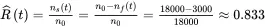
The total number of valves tested in the past three years is

The number of failed components is

According to Equation 1.3, an estimate of the valve reliability is

1.1.2 Probability of Time to Failure
Let random variable T denote the time to failure. Then, the reliability function at time t can be expressed as the probability that the component does not fail at time t, that is,
 (1.4)
(1.4)
Denote the cumulative distribution function (cdf) of T as F(t). The relationship between the cdf and the reliability is
 (1.5)
(1.5)
Further, denote the probability density function (pdf) of failure time T as f(t). Then, equation ( 1.5) can be rewritten as
 (1.6)
(1.6)
In all generality, the expected value or mean of the time to failure T is called the mean time to failure (MTTF), which is defined as
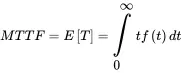 (1.7)
(1.7)
It is equivalent to
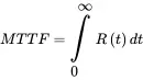 (1.8)
(1.8)
Another related concept is the mean time between failures (MTBF). MTBF is the average working time between two consecutive failures. The difference between MTBF and MTTF is that the former is used only in reference to a repairable item, while the latter is used for non-repairable items. However, MTBF is commonly used for both repairable and non-repairable items in practice.
The failure rate function or hazard rate function, denoted by h(t), is defined as the conditional probability of failure in the time interval [t, t+Δt] given that it has been working properly up to time t, which is given by
 (1.9)
(1.9)
Furthermore, the cumulative failure rate function, or cumulative hazard function, denoted by H(t), is given by
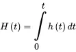 (1.10)
Example 1.2The failure time of a valve follows the exponential distribution with parameter h(t) (in arbitrary units of time-1). The value is new and functioning at time h(t). Calculate the reliability of the valve at time h(t) (in arbitrary units of time).
Solution
The pdf of the failure time of the valve is

The reliability function of the valve is given by

At time, the value of the reliability is
1.2 Component Reliability Modeling
As mentioned in the previous section, in reliability engineering, the time to failure of an item is a random variable. In this section, we briefly introduce several commonly used discrete and continuous distributions for component reliability modeling.
1.2.1 Discrete Probability Distributions
If random variable X can take only a finite number k of different values x1,x2,…,xk or an infinite sequence of different values x1,x2,…, the random variable X has a discrete probability distribution. The probability mass function (pmf) of X is defined as the function f such that for every real number x,
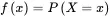 (1.11)
If x is not one of the possible values of X, then f(x)=0. If the sequence x1,x2,… includes all the possible values of X, then ∑if(xi)=1. The cdf is given by
 (1.12)
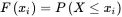
1.2.1.1 Binomial Distribution
Consider a machine that produces a defective item with probability p (0
1.14), shown in Figure 1.1. The random variable with this distribution is said to be a binomial random variable, with parameters n and p,
 (1.13)
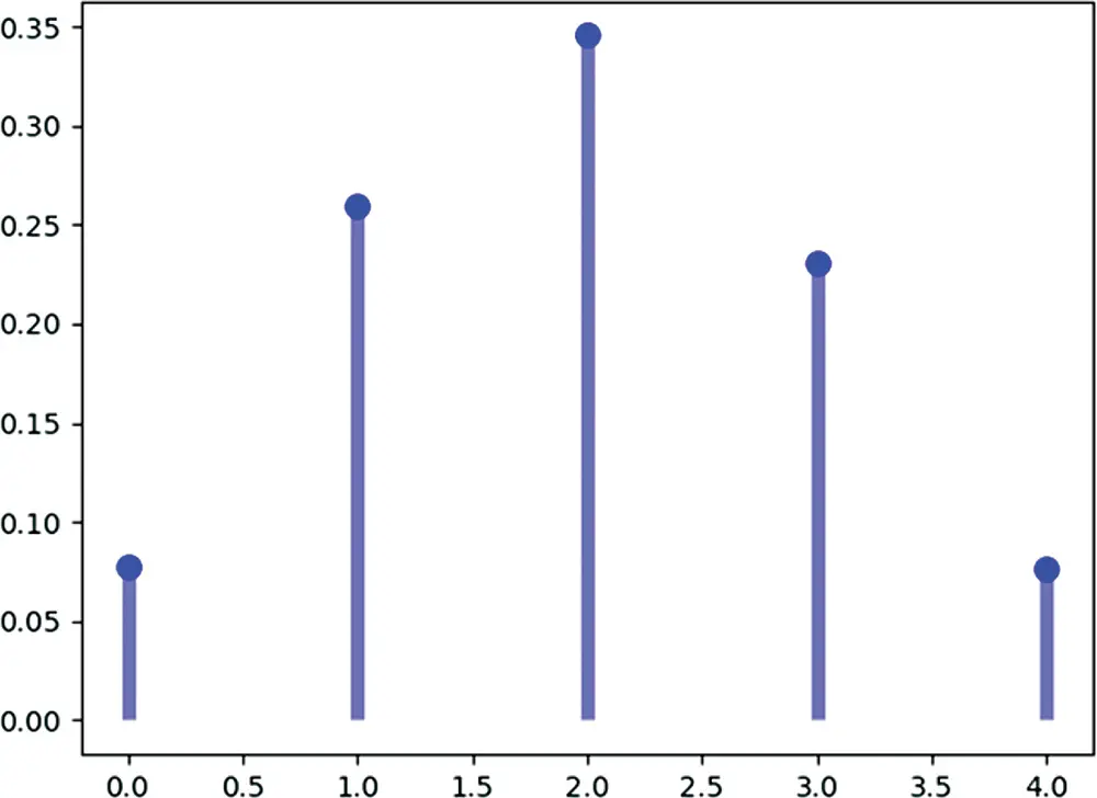
Figure 1.1 The pmf of the binomial distribution with n=5, p=0.4.
The pmf of the binomial distribution is
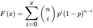 (1.14)
For a binomial distribution, the mean, μ, is given by
 (1.15)
and the variance, σ2, is given by
 (1.16)
1.2.1.2 Poisson Distribution
Poisson distribution is widely used in quality and reliability engineering. A random variable X has the Poisson distribution with parameter λ, λ>0, the pmf (shown in Figure 1.2) of X is as follows:
Читать дальшеИнтервал:
Закладка:
Похожие книги на «Reliability Analysis, Safety Assessment and Optimization»
Представляем Вашему вниманию похожие книги на «Reliability Analysis, Safety Assessment and Optimization» списком для выбора. Мы отобрали схожую по названию и смыслу литературу в надежде предоставить читателям больше вариантов отыскать новые, интересные, ещё непрочитанные произведения.


Обсуждение, отзывы о книге «Reliability Analysis, Safety Assessment and Optimization» и просто собственные мнения читателей. Оставьте ваши комментарии, напишите, что Вы думаете о произведении, его смысле или главных героях. Укажите что конкретно понравилось, а что нет, и почему Вы так считаете.