Neil McCartney - Properties for Design of Composite Structures
Здесь есть возможность читать онлайн «Neil McCartney - Properties for Design of Composite Structures» — ознакомительный отрывок электронной книги совершенно бесплатно, а после прочтения отрывка купить полную версию. В некоторых случаях можно слушать аудио, скачать через торрент в формате fb2 и присутствует краткое содержание. Жанр: unrecognised, на английском языке. Описание произведения, (предисловие) а так же отзывы посетителей доступны на портале библиотеки ЛибКат.
- Название:Properties for Design of Composite Structures
- Автор:
- Жанр:
- Год:неизвестен
- ISBN:нет данных
- Рейтинг книги:4 / 5. Голосов: 1
-
Избранное:Добавить в избранное
- Отзывы:
-
Ваша оценка:
Properties for Design of Composite Structures: краткое содержание, описание и аннотация
Предлагаем к чтению аннотацию, описание, краткое содержание или предисловие (зависит от того, что написал сам автор книги «Properties for Design of Composite Structures»). Если вы не нашли необходимую информацию о книге — напишите в комментариях, мы постараемся отыскать её.
A comprehensive guide to analytical methods and source code to predict the behavior of undamaged and damaged composite materials Properties for Design of Composite Structures: Theory and Implementation Using Software
Properties for Design of Composite Structures: Theory and Implementation Using Software
Properties for Design of Composite Structures — читать онлайн ознакомительный отрывок
Ниже представлен текст книги, разбитый по страницам. Система сохранения места последней прочитанной страницы, позволяет с удобством читать онлайн бесплатно книгу «Properties for Design of Composite Structures», без необходимости каждый раз заново искать на чём Вы остановились. Поставьте закладку, и сможете в любой момент перейти на страницу, на которой закончили чтение.
Интервал:
Закладка:
 (3.2)
(3.2)
Whatever the nature and arrangement of spherical particles in the cluster, Maxwell’s methodology considers the far-field when replacing the isotropic discrete particulate composite shown in Figure 3.1(a), that can just be enclosed by a sphere of radius b , by a homogeneous effective composite sphere of the same radius b embedded in the matrix as shown in Figure 3.1(b). There is no restriction on sizes, properties and locations of particles except that the equivalent effective medium is homogeneous and isotropic. Composites having statistical distributions of both size and properties can clearly be analysed.
3.2.2 Temperature Distribution for an Isolated Sphere Embedded in an Infinite Matrix
A set of spherical polar coordinates (r,θ,ϕ) is introduced having origin at the centre of the sphere of radius a . For steady-state conditions, the temperature distribution T(r,θ,ϕ) in the particle and surrounding matrix must satisfy Laplace’s equation, which is expressed in terms of spherical polar coordinates for the case where the temperature is independent of ϕ, namely,
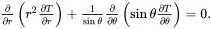 (3.3)
(3.3)
On the external boundary r→∞ a temperature distribution is imposed that would lead, in a homogeneous matrix material under steady-state conditions, to the following linear temperature distribution having a uniform gradient α
 (3.4)
(3.4)
At the particle/matrix interface r = a , the following conditions are imposed
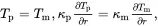 (3.5)
(3.5)
where both the temperature and the normal heat flux are assumed to be continuous across the interface, and where the isotropic thermal conductivities of particles and matrix are denoted by κpandκm, respectively. The temperature distribution T(r,θ) in the particle and matrix, satisfying ( 3.3), the condition at infinity and the interface conditions ( 3.5), is given by
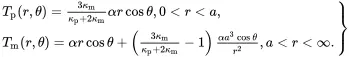 (3.6)
(3.6)
As x3=rcosθ, the temperature gradient is uniform within the particle. Any temperature T0 can be added to ( 3.6) without affecting the satisfaction of the interface conditions ( 3.5). As an infinite medium having a uniform temperature gradient is considered, it is inevitable that temperatures lower than absolute zero will be encountered. This physical absurdity can be avoided by assuming that the system is taken as a spherical region having a very large but finite radius, in which case T0 would be chosen large enough to ensure that the absolute temperature distribution is everywhere positive.
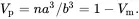
3.2.3 Maxwell’s Methodology for Estimating Conductivity
The first step of Maxwell’s approach considers the effect of embedding in the infinite isotropic matrix, an isolated cluster of isotropic spherical particles of different types that can be just contained within a sphere of radius b , as illustrated in Figure 3.1(a). The isotropic thermal conductivity of particles of type i is denoted by κp(i). The cluster is assumed to be effectively homogeneous regarding the distribution of particles, leading to an isotropic effective thermal conductivity κeff for the composite lying within the sphere of radius b . For a single particle, the matrix temperature distribution is perturbed from the distribution ( 3.4) to the distribution ( 3.6) that depends on particle geometry and properties. The perturbing effect in the matrix at large distances from the cluster of particles is estimated by superimposing the perturbations caused by each spherical particle, regarded as being isolated. The second step recognises that, at very large distances from the cluster, all the particles can be considered located at the origin that is chosen to be situated at the centre of one of the particles in the cluster. Thus, for the case of multiple phases, the approximate temperature distribution in the matrix at large distances from the cluster is given by the following generalisation of the second of relations ( 3.6):
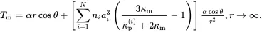 (3.7)
(3.7)
On using ( 3.1), this relation may be expressed in terms of the volume fractions so that
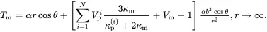 (3.8)
(3.8)
The third step involves replacing the composite having discrete particles lying within the sphere of radius b by a homogeneous spherical isotropic effective medium (see Figure 3.1(b)) having radius b and having the isotropic effective thermal conductivity κeff of the composite. On using ( 3.6), the temperature distribution in the matrix outside the sphere of effective medium having radius b is then given exactly, for a given value of κeff, by
 (3.9)
(3.9)
If the cluster in Figure 3.1(a) is represented accurately by the effective medium shown in Figure 3.1(b), then, at large distances from the cluster, the temperature distributions ( 3.8) and ( 3.9) should be identical, leading to the fourth step, where the perturbation terms in relations ( 3.8) and ( 3.9) are equated, so that
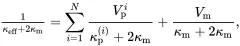 (3.10)
which is a ‘mixtures’ relation for the quantity 1/(κ+2κm). On using ( 3.1), the effective thermal conductivity may be estimated using
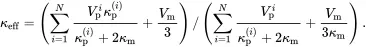 (3.11)
For multiphase composites, Hashin and Shtrikman [5, Equations ( 3.21)–( 3.23)] derived bounds for magnetic permeability, pointing out that they are analogous to bounds for effective thermal conductivity. Their conductivity bounds may be expressed in the following simpler form, having the same structure as the result ( 3.10) derived using Maxwell’s methodology
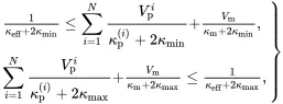 (3.12)
where κmin is the lowest value of conductivities for all phases, whereas κmax is the highest value.
3.3 Bulk Modulus and Thermal Expansion Coefficient
3.3.1 Spherical Particle Embedded in Infinite Matrix Subject to Pressure and Thermal Loading
Consider an isolated particle of radius a perfectly bonded to an infinite surrounding matrix, subject to a pressure p applied at infinity and a uniform temperature change ΔT from the stress-free temperature at which the stresses and strains in particle and matrix are zero. The displacement field in the particle and surrounding matrix is purely radial so that displacement components (ur,uθ,uϕ), referred to a set of spherical polar coordinates ( r , θ , ϕ ) with origin at the particle centre, are of the form
Читать дальшеИнтервал:
Закладка:
Похожие книги на «Properties for Design of Composite Structures»
Представляем Вашему вниманию похожие книги на «Properties for Design of Composite Structures» списком для выбора. Мы отобрали схожую по названию и смыслу литературу в надежде предоставить читателям больше вариантов отыскать новые, интересные, ещё непрочитанные произведения.


Обсуждение, отзывы о книге «Properties for Design of Composite Structures» и просто собственные мнения читателей. Оставьте ваши комментарии, напишите, что Вы думаете о произведении, его смысле или главных героях. Укажите что конкретно понравилось, а что нет, и почему Вы так считаете.