Pedro Domingos - The Master Algorithm - How the Quest for the Ultimate Learning Machine Will Remake Our World

The origins of MCMC go all the way back to the Manhattan Project, when physicists needed to estimate the probability that neutrons would collide with atoms and set off a chain reaction. But in more recent decades, it has sparked such a revolution that it’s often considered one of the most important algorithms of all time. MCMC is good not just for computing probabilities but for integrating any function. Without it, scientists were limited to functions they could integrate analytically, or to well-behaved, low-dimensional integrals they could approximate as a series of trapezoids. With MCMC, they’re free to build complex models, knowing the computer will do the heavy lifting. Bayesians, for one, probably have MCMC to thank for the rising popularity of their methods more than anything else.

On the downside, MCMC is often excruciatingly slow to converge, or fools you by looking like it’s converged when it hasn’t. Real probability distributions are usually very peaked, with vast wastelands of minuscule probability punctuated by sudden Everests. The Markov chain then converges to the nearest peak and stays there, leading to very biased probability estimates. It’s as if the drunkard followed the scent of alcohol to the nearest tavern and stayed there all night, instead of wandering all around the city like we wanted him to. On the other hand, if instead of using a Markov chain we just generated independent samples, like simpler Monte Carlo methods do, we’d have no scent to follow and probably wouldn’t even find that first tavern; it would be like throwing darts at a map of the city, hoping they land smack dab on the pubs.

Inference in Bayesian networks is not limited to computing probabilities. It also includes finding the most probable explanation for the evidence, such as the disease that best explains the symptoms or the words that best explain the sounds Siri heard. This is not the same as just picking the most probable word at each step, because words that are individually likely given their sounds may be unlikely to occur together, as in the “Call the please” example. However, similar kinds of algorithms also work for this task (and they are, in fact, what most speech recognizers use). Most importantly, inference includes making the best decisions, guided not just by the probabilities of different outcomes but also by the corresponding costs (or utilities, to use the technical term). The cost of ignoring an e-mail from your boss asking you to do something by tomorrow is much greater than the cost of seeing a piece of spam, so often it’s better to let an e-mail through even if it does seem fairly likely to be spam.

Driverless cars and other robots are a prime example of probabilistic inference in action. As the car drives around, it simultaneously builds up a map of the territory and figures out its location on it with increasing certainty. According to a recent study, London taxi drivers grow a larger posterior hippocampus, a brain region involved in memory and map making, as they learn the layout of the city. Perhaps they use similar probabilistic inference algorithms, with the notable difference that in the case of humans, drinking doesn’t seem to help.

Learning the Bayesian way

Now that we know how to (more or less) solve the inference problem, we’re ready to learn Bayesian networks from data, because for Bayesians learning is just another kind of probabilistic inference. All you have to do is apply Bayes’ theorem with the hypotheses as the possible causes and the data as the observed effect:

P(hypothesis | data) = P(hypothesis) × P(data | hypothesis) / P(data)

The hypothesis can be as complex as a whole Bayesian network, or as simple as the probability that a coin will come up heads. In the latter case, the data is just the outcome of a series of coin flips. If, say, we obtain seventy heads in a hundred flips, a frequentist would estimate the probability of heads as 0.7. This is justified by the so-called maximum likelihood principle: of all the possible probabilities of heads, 0.7 is the one under which seeing seventy heads in a hundred flips is most likely. The likelihood of a hypothesis is P(data | hypothesis) , and the principle says we should pick the hypothesis that maximizes it. Bayesians do something more subtle, though. They point out that we never know for sure which hypothesis is the true one, and so we shouldn’t just pick one hypothesis, like a value of 0.7 for the probability of heads; rather, we should compute the posterior probability of every possible hypothesis and entertain all of them when making predictions. The sum of the probabilities of all the hypotheses must be one, so if one becomes more likely, the others become less. For a Bayesian, in fact, there is no such thing as the truth; you have a prior distribution over hypotheses, after seeing the data it becomes the posterior distribution, as given by Bayes’ theorem, and that’s all.

This is a radical departure from the way science is usually done. It’s like saying, “Actually, neither Copernicus nor Ptolemy was right; let’s just predict the planets’ future trajectories assuming Earth goes round the sun and vice versa and average the results.”

Of course, it’s a weighted average, the weight of a hypothesis being its posterior probability, so a hypothesis that explains the data better will count for more. Still, as the joke goes, being Bayesian means never having to say you’re certain.

Needless to say, carrying around a multitude of hypotheses instead of just one is a huge pain. In the case of learning a Bayesian network, we’re supposed to make predictions by averaging over all possible Bayesian networks, including all possible graph structures and all possible parameter values for each structure. In some cases, we can compute the average over parameters in closed form, but with varying structures we’re out of luck. We have to resort to, for example, doing MCMC over the space of networks, jumping from one possible network to another as the Markov chain progresses. Combine all this complexity and computational cost with Bayesians’ controversial notion that there’s really no such thing as objective reality, and it’s not hard to see why frequentism has dominated science for the last century.

There’s a saving grace, however, and some major reasons to prefer the Bayesian way. The saving grace is that, most of the time, almost all hypotheses wind up with a tiny posterior probability, and we can safely ignore them. In fact, just considering the single most probable hypothesis is usually a very good approximation. Suppose our prior distribution for the coin flip problem is that all probabilities of heads are equally likely. The effect of seeing the outcomes of successive flips is to concentrate the distribution more and more on the hypotheses that best agree with the data. For example, if h ranges over the possible probabilities of heads and a coin comes out heads 70 percent of the time, we’ll see something like this:

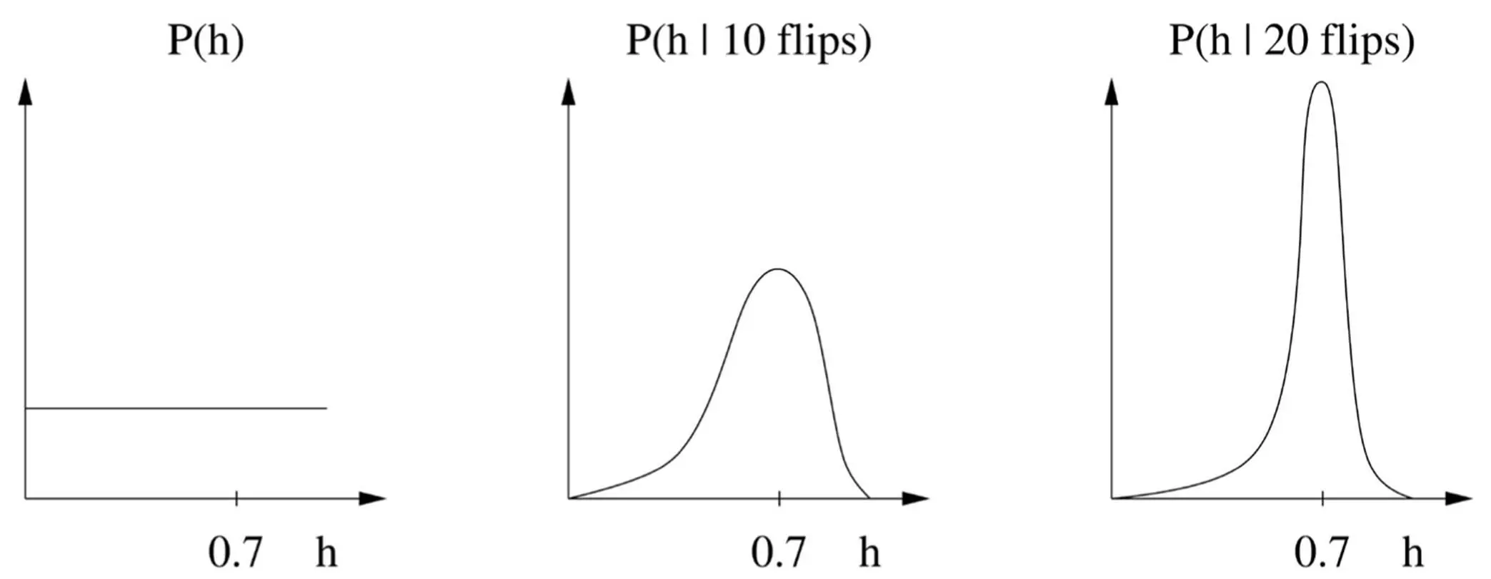
The posterior after each flip becomes the prior for the next flip, and flip by flip, we become increasingly certain that h = 0.7. If we just take the single most probable hypothesis ( h = 0.7 in this case), the Bayesian approach becomes quite similar to the frequentist one, but with one crucial difference: Bayesians take the prior P(hypothesis) into account, not just the likelihood P(data | hypothesis) . (The data prior P(data) can be ignored because it’s the same for all hypotheses and therefore doesn’t affect the choice of winner.) If we’re willing to assume that all hypotheses are equally likely a priori, the Bayesian approach now reduces to the maximum likelihood principle. So Bayesians can say to frequentists: “See, what you do is a special case of what we do, but at least we make our assumptions explicit.” And if the hypotheses are not equally likely a priori, maximum likelihood’s implicit assumption that they are leads to the wrong answers.