Zhuming Bi - Computer Aided Design and Manufacturing
Здесь есть возможность читать онлайн «Zhuming Bi - Computer Aided Design and Manufacturing» — ознакомительный отрывок электронной книги совершенно бесплатно, а после прочтения отрывка купить полную версию. В некоторых случаях можно слушать аудио, скачать через торрент в формате fb2 и присутствует краткое содержание. Жанр: unrecognised, на английском языке. Описание произведения, (предисловие) а так же отзывы посетителей доступны на портале библиотеки ЛибКат.
- Название:Computer Aided Design and Manufacturing
- Автор:
- Жанр:
- Год:неизвестен
- ISBN:нет данных
- Рейтинг книги:3 / 5. Голосов: 1
-
Избранное:Добавить в избранное
- Отзывы:
-
Ваша оценка:
Computer Aided Design and Manufacturing: краткое содержание, описание и аннотация
Предлагаем к чтению аннотацию, описание, краткое содержание или предисловие (зависит от того, что написал сам автор книги «Computer Aided Design and Manufacturing»). Если вы не нашли необходимую информацию о книге — напишите в комментариях, мы постараемся отыскать её.
Computer Aided Design and Manufacturing being uniquely structured to classify and align engineering disciplines and computer aided technologies from the perspective of the design needs in whole product life cycles, utilizing a comprehensive Solidworks package (add-ins, toolbox, and library) to showcase the most critical functionalities of modern computer aided tools, and presenting real-world design projects and case studies so that readers can gain CAD and CAM problem-solving skills upon the CAD/CAM theory.
is an ideal textbook for undergraduate and graduate students in mechanical engineering, manufacturing engineering, and industrial engineering. It can also be used as a technical reference for researchers and engineers in mechanical and manufacturing engineering or computer-aided technologies.
Computer Aided Design and Manufacturing — читать онлайн ознакомительный отрывок
Ниже представлен текст книги, разбитый по страницам. Система сохранения места последней прочитанной страницы, позволяет с удобством читать онлайн бесплатно книгу «Computer Aided Design and Manufacturing», без необходимости каждый раз заново искать на чём Вы остановились. Поставьте закладку, и сможете в любой момент перейти на страницу, на которой закончили чтение.
Интервал:
Закладка:
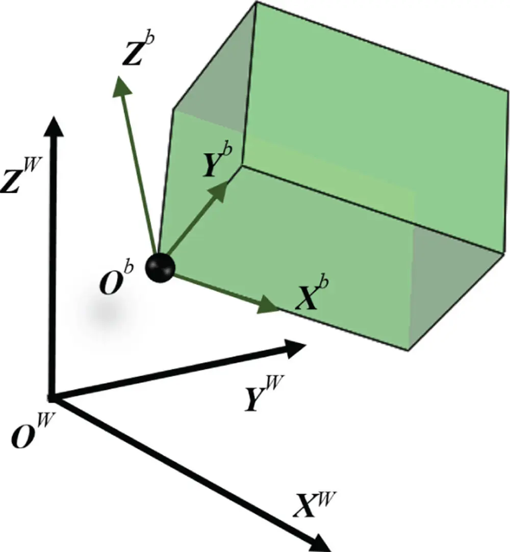
Figure 2.9Object coordinate system in a world coordinate system.
In Figure 2.9, a reference origin 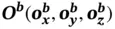 is used to represent the position of the object with respect to the world coordinate system ( O w− X w Y w Z w) and the orientation of the object is represented by three unit vectors ( X b, Y b, Z b). Furthermore, a homogeneous coordinate ( x , y , z , h ) and the corresponding 4 by 4 homogenous matrix [ T] 4x4in Eq. (2.4) are widely used to facilitate the matrix manipulations for the coordinate transformation of objects:
(2.4) 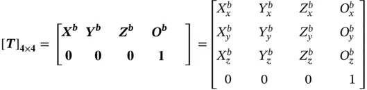
where [ T] 4 × 4is the homogenous matrix for the representation of an object CS { O b− X b Y b Z b} in the world coordinate system ( O w− X w Y w Z w).
Note that the homogenous matrix in Eq. (2.4) includes six independent variables: three for the position and the rest for the orientation.
A homogenous transformation matrix can be generalized to deal with any transformation of objects in a coordinate system. Figure 2.10shows the generalized matrix of homogeneous transformation. The elements of the matrix in different fields affect the transformation of an object in different ways. For examples, the elements ( a , e , j ) scale the coordinates of x , y , and z , the elements ( p , q , r ) translate the coordinates of x , y , and z , and the element s gives an overall inverse scale of the object.
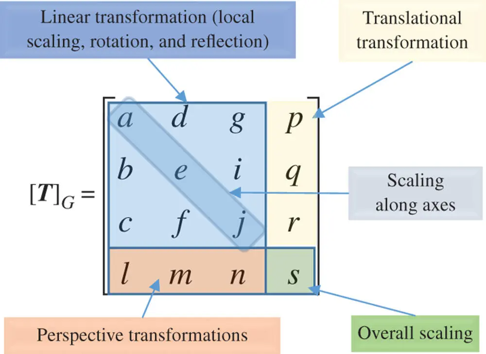
Figure 2.10Impacts of elements in a generalized homogeneous matrix.
The generic homogeneous matrix [ T] Gcan be customized to implement some common coordinate transformations of an object. For example, the translation matrix [ T] TRof an object can be simplified as
(2.5) 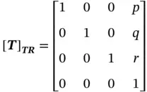
where [ T] TRis the 3D translation matrix and p , q , r are the translational distances of a point from its original position along the x, y, and zaxes, respectively.
The scaling matrix [ T] SCof a 3D object can be defined as
(2.6) 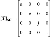
where [ T] SCis the 3D scaling matrix and a , e , j are the scaling factors along the x, y, and zaxes, respectively.
Example 2.1
Given a cube with the size of 1 × 1 × 1 at its origin in Figure 2.11, determine the vertices of the object after the lengths along the x, y, zaxes are scaled up by 2, 3, and 1, respectively.
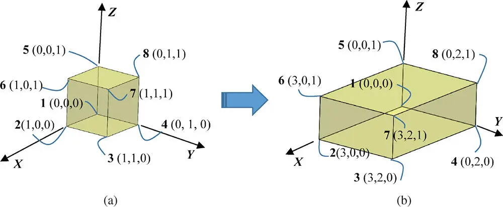
Figure 2.11Example of a scaling matrix of a 3D object. (a) Before transformation. (b) After transformation.
Solution
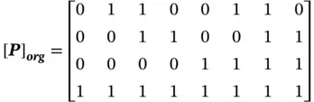
Before the transformation, the set of eight vertices (1, 2, …, 8) in their homogeneous coordinates is written as
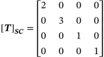
Using the given scales along the x , y , z axes, the scaling matrix Eq. (2.6) is given as
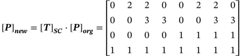
Therefore, the set of vertices of the object after scaling transformation can be found as
A 3D reflection refers to a transformation of mirroring an object about a specified plane. A reflection transformation matrix can be treated as a special case of a scaling matrix, where the scale of the corresponding axis of the reflected coordinate is set as a negative value of −1. Note that the axis for the reflection is aligned with the normal reflecting or mirroring plane. Therefore, the reflection coordination transformations about YZ, XZ, and XYplanes are expressed by [ T] RE_YZ, [ T] RE_XZ, and [ T] RE_XZ, respectively, as follows:
(2.7) 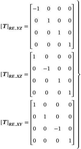
Example 2.2
Figure 2.12a shows an object in the coordinate system ( O‐XYZ) with the specified set of vertices as follows:
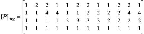
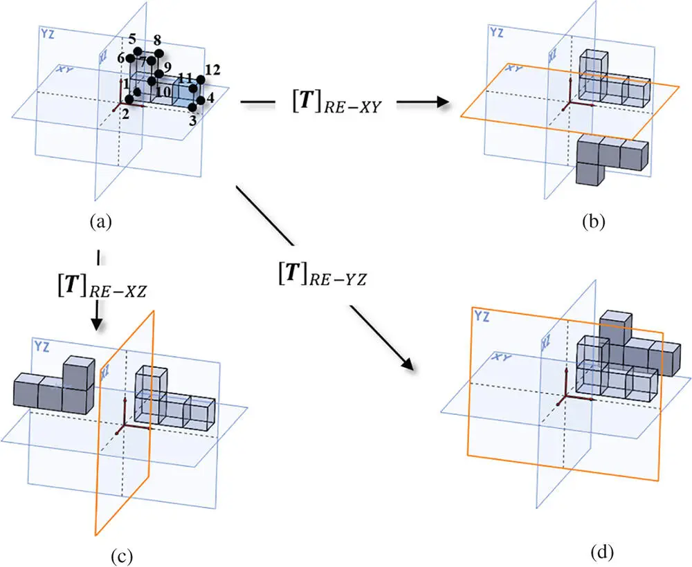
Figure 2.12Reflection coordinate transformation matrices of an object. (a) Object at the original position. (b) Reflected object about the XYplane. (c) Reflected object about the YZplane. (d) Reflected object about the YZplane.
Determine the reflected objects about the XY, YZ, XZplanes, respectively.
Solution
Using Eq. (2.7), the vertices of the reflected objects about the XY, YZ, XZplanes are determined and illustrated in Figure 2.12b to d, respectively. Taking as an example determination of the reflected object about the XY plane,

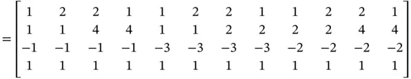
where [ T] RE − XYis given in Eq. (2.7) for the reflected object about the XYplane.
Читать дальшеИнтервал:
Закладка:
Похожие книги на «Computer Aided Design and Manufacturing»
Представляем Вашему вниманию похожие книги на «Computer Aided Design and Manufacturing» списком для выбора. Мы отобрали схожую по названию и смыслу литературу в надежде предоставить читателям больше вариантов отыскать новые, интересные, ещё непрочитанные произведения.


Обсуждение, отзывы о книге «Computer Aided Design and Manufacturing» и просто собственные мнения читателей. Оставьте ваши комментарии, напишите, что Вы думаете о произведении, его смысле или главных героях. Укажите что конкретно понравилось, а что нет, и почему Вы так считаете.