Samprit Chatterjee - Handbook of Regression Analysis With Applications in R

Figure 1.2gives a graphical representation of least squares that is based on Figure 1.1. Now the true regression line is represented by the gray line, and the solid black line is the estimated regression line, designed to estimate the (unknown) gray line as closely as possible. For any choice of estimated parameters , the estimated expected response value given the observed predictor values equals

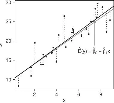
FIGURE 1.2: Least squares estimation for the simple linear regression model, using the same data as in Figure 1.1. The gray line corresponds to the true regression line, the solid black line corresponds to the fitted least squares line (designed to estimate the gray line), and the lengths of the dotted lines correspond to the residuals. The sum of squared values of the lengths of the dotted lines is minimized by the solid black line.

and is called the fitted value. The difference between the observed value and the fitted value is called the residual, the set of which is represented by the signed lengths of the dotted lines in Figure 1.2. The least squares regression line minimizes the sum of squares of the lengths of the dotted lines; that is, the ordinary least squares (OLS) estimates minimize the sum of squares of the residuals.

In higher dimensions ( ), the true and estimated regression relationships correspond to planes ( ) or hyperplanes ( ), but otherwise the principles are the same. Figure 1.3illustrates the case with two predictors. The length of each vertical line corresponds to a residual (solid lines refer to positive residuals, while dashed lines refer to negative residuals), and the (least squares) plane that goes through the observations is chosen to minimize the sum of squares of the residuals.

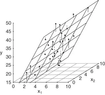
FIGURE 1.3: Least squares estimation for the multiple linear regression model with two predictors. The plane corresponds to the fitted least squares relationship, and the lengths of the vertical lines correspond to the residuals. The sum of squared values of the lengths of the vertical lines is minimized by the plane.

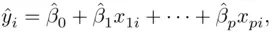
The linear regression model can be written compactly using matrix notation. Define the following matrix and vectors as follows:

The regression model (1.1)is then

(1.3)

The normal equations [which determine the minimizer of 1.2] can be shown (using multivariate calculus) to be

which implies that the least squares estimates satisfy

(1.4)

The fitted values are then

(1.5)

where is the so‐called “hat” matrix (since it takes to ). The residuals thus satisfy

(1.6)

or

The least squares criterion will not necessarily yield sensible results unless certain assumptions hold. One is given in (1.1)— the linear model should be appropriate. In addition, the following assumptions are needed to justify using least squares regression.

1 The expected value of the errors is zero ( for all ). That is, it cannot be true that for certain observations the model is systematically too low, while for others it is systematically too high. A violation of this assumption will lead to difficulties in estimating . More importantly, this reflects that the model does not include a necessary systematic component, which has instead been absorbed into the error terms.

2 The variance of the errors is constant ( for all ). That is, it cannot be true that the strength of the model is greater for some parts of the population (smaller ) and less for other parts (larger ). This assumption of constant variance is called homoscedasticity, and its violation (nonconstant variance) is called heteroscedasticity. A violation of this assumption means that the least squares estimates are not as efficient as they could be in estimating the true parameters, and better estimates are available. More importantly, it also results in poorly calibrated confidence and (especially) prediction intervals.

3 The errors are uncorrelated with each other. That is, it cannot be true that knowing that the model underpredicts (for example) for one particular observation says anything at all about what it does for any other observation. This violation most often occurs in data that are ordered in time (time series data), where errors that are near each other in time are often similar to each other (such time‐related correlation is called autocorrelation). Violation of this assumption means that the least squares estimates are not as efficient as they could be in estimating the true parameters, and more importantly, its presence can lead to very misleading assessments of the strength of the regression.