Peter M. B. Cahusac - Evidence-Based Statistics

Perhaps the most concentrated account of likelihood, given in just a few pages, is by Edwards in a 2015 entry for an encyclopaedia [16]. There are a number of accessible research papers. Those by Goodman [17–21] (one of these jointly with Royall), and Dixon and Glover [22, 23] are exemplary in explaining and demonstrating a range of evidential techniques.

Together with the data, s tatistical hypotheses and statistical model s are essential components for us to be able to draw inferences. Hypotheses and models provide an adequate probabilistic explanation of the process by which the observed data were generated. By statistical hypothesis, we mean attributing a specified quantitative or qualitative value to an identified parameter of interest within the statistical model. A simple statistical hypothesis specifies a particular value. For example, the null hypothesis for a measured difference between two populations might be exactly 0. A hypothesis may also be a range of values, known as a composite hypothesis, for example the direction of difference in a measurement of two populations (e.g. A > B). By statistical model, we mean the mathematical assumptions we make about how sample data (and similar samples from the same population) were generated. Typically, a model is a convenient simplification of a more complex reality. Statistical inference and estimation are conditional on a model. For example, in comparing heights of malnourished and well-nourished adults, our model could assume that the measurements are normally distributed. We might specify two simple hypotheses to be compared, for example: the null of 0 difference and a population mean difference of more than 3 cm between the two populations. The distinction between hypothesis and model is not absolute since it is possible to consider one of these components to be part of the model on one occasion and then contested as a hypothesis on another. Hence, our model assumption of normally distributed data could itself be questioned by becoming a hypothesis.

There are three main statistical approaches to data analysis. These are neatly summarized by Royall's three questions that follow the collection and analysis of some data [24]:

1 What should I do?

2 What should I believe?

3 How should I interpret the evidence?

They describe the different ways in which the data are analyzed and interpreted. Each approach is important within their specific domain. The first of these is pragmatic, where a decision must be made on the basis of the analysis. It represents the frequentist approaches of statistical tests and hypothesis testing. Typically, either the null hypothesis is rejected (evidence for an effect is found) or not rejected (insufficient evidence found). The decision is based upon a critical probability, usually .05. The significance testing approach measures the strength of evidence against the null hypothesis by the diminutiveness of a calculated probability of obtaining the data (or more extreme) assuming the null hypothesis is true. This probability is known as a p value.

The second approach represents the strength of belief for a specified hypothesis. It too is based upon probability and is conditioned by the probability of the hypothesis prior to the collection of the data. If the prior probability is known, then the calculation using Bayes' theorem logically provides the (posterior) probability for the specified hypothesis.

The third approach also uses probability but provides objective evidence which is expressed as the likelihood for one hypothesis versus another in the form of a LR. The LR is not a probability but a relative measure of evidence for competing hypotheses. The technical meaning of the word ‘likelihood’ in statistics is very similar to its use in common parlance by non-statisticians. For example we might say, seeing dark clouds in the sky, ‘there is a greater likelihood for rain than sunshine this afternoon’.

When the LR is transformed into the natural logarithm, it is known as the support , denoted S . The support quantifies the comparative evidence on a scale of −∞ to +∞, with midpoint 0 representing no evidence in favour of either hypothesis. Unlike the use of p , S is a graded measure of evidence without clear cutoffs or thresholds.

If the collected data are not strongly influenced by prior considerations, it is somewhat reassuring that the three approaches usually reach the same conclusion. However, it is not difficult to find examples of where the likelihood evidence points one way and the hypothesis testing decision points the other (see Section 3.7, and de Winter and Cahusac [25], p. 89 and Dienes [6], p. 127)

In advocating the evidential approach, Royall wrote in 2004 ‘Statistics today is in a conceptual and theoretical mess. The discipline is divided into two rival camps, the frequentists and the Bayesians, and neither camp offers the tools that science needs for objectively representing and interpreting statistical data as evidence’ [24], p. 127.

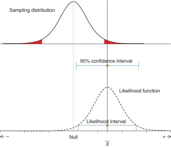
In making sense of data and to make inferences, it is natural to consider different rival hypotheses to explain how such a set of observations arose. Significance testing uses a single hypothesis to test, typically the null hypothesis. The top of Figure 1.1illustrates the typical situation when testing a sample mean. The sampling distribution for the mean is located over the null value, see vertical dashed line down to the horizontal axis. The sample mean indicated by the continuous vertical line lies in the shaded rejection region. The shaded region represents 5% of the area under the sampling distribution curve, with 2.5% in each tail. Significance testing states a pre-specified significance level α , typically this is 5%. Since the value for the sample mean lies within the shaded area, we can say that p < .05 and we reject the null hypothesis given our α .

Estimation, a key element in statistical analysis, has often been ignored in the face of dichotomous decisions reached from statistical tests. If results are reported as non-significant, it is assumed that there is no effect or difference between population parameters. Alternatively, highly significant results based on large samples are assumed to represent large effects. The increased use of confidence intervals [26] is a great improvement that allows us to see how large or small the magnitude of the effects are, and hence whether they are of practical/clinical importance. These advances have increased the credibility of well-reported studies and facilitated our understanding of research results. The confidence interval is illustrated in the middle portion of Figure 1.1. This is centred on the sample mean (shown by the end-stopped line) and gives a range of plausible values for the population mean [26]. The interval has a frequentist interpretation: 95% of such intervals, calculated from random samples taken from the population of interest, will contain the population statistic. The confidence interval focusses our attention on the obtained sample mean value, and the 95% limits indicate how far this value is from parameter values of interest, especially the null. The interval helps us determine whether the data we have is of practical importance.

Figure 1.1 From sampling distribution to likelihood function. The top curve shows the sampling distribution used for testing statistical significance. It is centred on the null hypothesis value (often 0) and the standard error used to calculate the curve comes from the observed data. Below this in the middle is shown the 95% confidence interval. This uses the sample mean and standard error from the observed data. At the bottom shows the likelihood function, within which is plotted the S -2 likelihood function. Both the likelihood function and the likelihood interval use the observed data like the confidence interval.