George Acquaah - Principles of Plant Genetics and Breeding
Здесь есть возможность читать онлайн «George Acquaah - Principles of Plant Genetics and Breeding» — ознакомительный отрывок электронной книги совершенно бесплатно, а после прочтения отрывка купить полную версию. В некоторых случаях можно слушать аудио, скачать через торрент в формате fb2 и присутствует краткое содержание. Жанр: unrecognised, на английском языке. Описание произведения, (предисловие) а так же отзывы посетителей доступны на портале библиотеки ЛибКат.
- Название:Principles of Plant Genetics and Breeding
- Автор:
- Жанр:
- Год:неизвестен
- ISBN:нет данных
- Рейтинг книги:5 / 5. Голосов: 1
-
Избранное:Добавить в избранное
- Отзывы:
-
Ваша оценка:
Principles of Plant Genetics and Breeding: краткое содержание, описание и аннотация
Предлагаем к чтению аннотацию, описание, краткое содержание или предисловие (зависит от того, что написал сам автор книги «Principles of Plant Genetics and Breeding»). Если вы не нашли необходимую информацию о книге — напишите в комментариях, мы постараемся отыскать её.
Organizes topics to reflect the stages of an actual breeding project Incorporates the most recent technologies in the field, such as CRSPR genome edition and grafting on GM stock Includes numerous illustrations and end-of-chapter self-assessment questions, key references, suggested readings, and links to relevant websites Features a companion website containing additional artwork and instructor resources
offers researchers and professionals an invaluable resource and remains the ideal textbook for advanced undergraduates and graduates in plant science, particularly those studying plant breeding, biotechnology, and genetics.
Principles of Plant Genetics and Breeding — читать онлайн ознакомительный отрывок
Ниже представлен текст книги, разбитый по страницам. Система сохранения места последней прочитанной страницы, позволяет с удобством читать онлайн бесплатно книгу «Principles of Plant Genetics and Breeding», без необходимости каждый раз заново искать на чём Вы остановились. Поставьте закладку, и сможете в любой момент перейти на страницу, на которой закончили чтение.
Интервал:
Закладка:
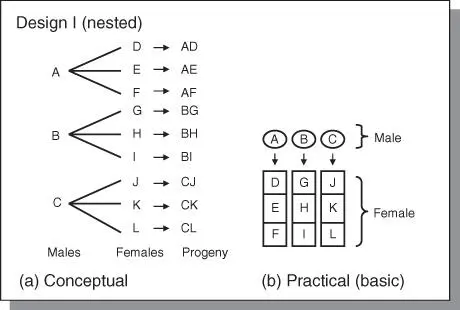
Figure 4.5The North Carolina Design I. (a) This design is a nested arrangement of genotypes for crossing in which no male is involved in more than one cross. (b) A practical layout in the field.
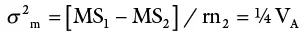
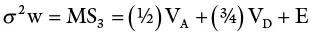
The total variance is partitioned as follows:
| Source | df | MS | EMS |
| Males | n−1 | MS 1 | σ 2w + rσ 2 flm+ rfσ 2 m |
| Females | n 1(n 2– 1) | MS 2 | σ 2w + rσ 2 flm |
| Within progenies | n 1n 2(r − 1) | MS 3 | σ 2w |

This design is most widely used in animal studies. In plants, it has been extensively used in maize breeding for estimating genetic variances.
North carolina design II
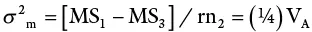
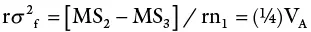
In this design, each member of a group of parents used as males is mated to each member of another group of parents used as females. Design IIis a factorial mating scheme similar to Design I ( Figure 4.6). It is used to evaluate inbred lines for combining ability. The design is most adapted to plants that have multiple flowers so that each plant can be used repeatedly as both male and female. Blocking is used in this design to allow all the mating involving a single group of males to a single group of females to be kept intact as a unit. The design is essentially a 2‐way ANOVA in which the variation may be partitioned into difference between males and females and their interaction. The ANOVA is as follows:
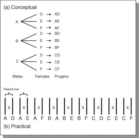
Figure 4.6North Carolina Design II. (a) This is a factorial design. (b) Paired rows may be used in the nursery for factorial mating of plants.
| Source | df | MS | EMS |
| Males | n 1– 1 | MS 1 | σ 2w + rσ 2 mf+ rnσ 2 m |
| Females | n 2– 1 | MS 2 | σ 2w + rσ 2 mf+ rn 1σ 2 f |
| Males × females | (n 1– 1)(n 2– 1) | MS 3 | σ 2w + rσ 2 mf |
| Within progenies | n 1n 2(r − 1) | MS 4 | σ 2w |
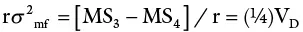

The design also allows the breeder to measure not only GCA but also SCA.
North carolina design III
In this design, a random sample of F 2plants is backcrossed to the two inbred lines from which the F 2was descended. It is considered the most powerful of all the three NC designs. However, it was made more powerful by the modifications made by Kearsey and Jinks that adds a third tester (not just the two inbreds) ( Figure 4.7). The modification is called the triple test crossand is capable of testing for non‐allelic (epistatic) interactions that the other designs cannot, and also estimate additive and dominance variance.
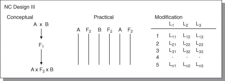
Figure 4.7North Carolina Design III. The conventional form (a), the practical layout (b), and the modification (c) are shown.
Diallele cross
A complete diallele matingdesign is one that allows the parents to be crossed in all possible combinations, including selfs and reciprocals. This is the kind of mating scheme required to achieve Hardy‐Weinberg equilibrium in a population. However, in practice, a diallele with selfs and reciprocals is neither practical nor useful for several reasons. Selfing does not contribute to recombination of genes between parents. Furthermore, recombination is achieved by crossing in one direction, making reciprocals unnecessary. Because of the extensive mating patterns, the number of parents that can be mated this way is limited. For p entries, a complete diallele will generate p 2crosses. Without selfs and reciprocals, the number is p(p − 1)/2 crosses.
When the number of entries is large, a partial diallele matingdesign, which allows all parents to be mated to some but not all other parents in the set, is used. A diallele designis most commonly used to estimate combining abilities (both general and specific). It is also widely used for developing breeding populations for recurrent selection.
Nursery arrangements for application of complete and partial diallele are varied. Because a large number of crosses are made, diallele mating takes a large amount of space, seed, labor, and time to conduct. Because all possible pairs are contained in one half of a symmetric Latin square, this design may be used to address some of the space needs.
There are four basic methods developed by Griffing that vary in either the omission of parents or the omission of reciprocals in the crosses. The number of progeny families (pf) for methods 1 through 4 are: pf = n 2, pf = ½ n(n + 1), pf = n(n − 1), and pf = ½ n(n − 1), respectively. The ANOVA for method 4, for example, is as follows:
| Source | dr | EMS |
| GCA | n 1− 1 | σ 2e + rσ 2 g+ r(n − 2)σ 2 |
| SCA | [n(n − 3)]/2 | σ 2e + rσ 2 g |
| Reps × Crosses | (r − 1){[n(n − 1)/2] − 1} | σ 2e |
Comparative evaluation of mating designs
Hill, Becker, and Tigerstedt roughly summarized these mating designs in two ways:
1 In terms of coverage of the population: BIPs > NCM‐I > Polycross > NCM‐III > NCM‐II > diallele, in that order of decreasing effectiveness.
2 In terms of amount of information: Diallele > NCM‐II > NCM‐II > NCM‐I > BIPs.
The diallele mating design is the most important for GCA and SCA. These researchers emphasized that it is not the mating design per se, but rather the breeder who breeds a new cultivar. The implication is that the proper choice and use of a mating design will provide the most valuable information for breeding.
4.3 The genetic architecture of quantitative traits
Molecular quantitative genetics mainly focuses on evaluating the coupling association of the polymorphic DNA sites with the phenotypic variations of quantitative and complex traits. In addition, whereas classical quantitative genetics deals with the holistic status of all genes, molecular quantitative genetics dissects the genetic architectures of quantitative genes (concerned with the analytical status of the major genes and holistic status of the minor genes).
Читать дальшеИнтервал:
Закладка:
Похожие книги на «Principles of Plant Genetics and Breeding»
Представляем Вашему вниманию похожие книги на «Principles of Plant Genetics and Breeding» списком для выбора. Мы отобрали схожую по названию и смыслу литературу в надежде предоставить читателям больше вариантов отыскать новые, интересные, ещё непрочитанные произведения.


Обсуждение, отзывы о книге «Principles of Plant Genetics and Breeding» и просто собственные мнения читателей. Оставьте ваши комментарии, напишите, что Вы думаете о произведении, его смысле или главных героях. Укажите что конкретно понравилось, а что нет, и почему Вы так считаете.