William M. White - Geochemistry
Здесь есть возможность читать онлайн «William M. White - Geochemistry» — ознакомительный отрывок электронной книги совершенно бесплатно, а после прочтения отрывка купить полную версию. В некоторых случаях можно слушать аудио, скачать через торрент в формате fb2 и присутствует краткое содержание. Жанр: unrecognised, на английском языке. Описание произведения, (предисловие) а так же отзывы посетителей доступны на портале библиотеки ЛибКат.
- Название:Geochemistry
- Автор:
- Жанр:
- Год:неизвестен
- ISBN:нет данных
- Рейтинг книги:5 / 5. Голосов: 1
-
Избранное:Добавить в избранное
- Отзывы:
-
Ваша оценка:
Geochemistry: краткое содержание, описание и аннотация
Предлагаем к чтению аннотацию, описание, краткое содержание или предисловие (зависит от того, что написал сам автор книги «Geochemistry»). Если вы не нашли необходимую информацию о книге — напишите в комментариях, мы постараемся отыскать её.
, undergraduate and graduate students will find each of the core principles of geochemistry covered. From defining key principles and methods to examining Earth’s core composition and exploring organic chemistry and fossil fuels, this definitive edition encompasses all the information needed for a solid foundation in the earth sciences for beginners and beyond.
For researchers and applied scientists, this book will act as a useful reference on fundamental theories of geochemistry, applications, and environmental sciences. The new edition includes new chapters on the geochemistry of the Earth’s surface (the “critical zone”), marine geochemistry, and applied geochemistry as it relates to environmental applications and geochemical exploration.
● A review of the fundamentals of geochemical thermodynamics and kinetics, trace element and organic geochemistry
● An introduction to radiogenic and stable isotope geochemistry and applications such as geologic time, ancient climates, and diets of prehistoric people
● Formation of the Earth and composition and origins of the core, the mantle, and the crust
● New chapters that cover soils and streams, the oceans, and geochemistry applied to the environment and mineral exploration
In this foundational look at geochemistry, new learners and professionals will find the answer to the essential principles and techniques of the science behind the Earth and its environs.
Geochemistry — читать онлайн ознакомительный отрывок
Ниже представлен текст книги, разбитый по страницам. Система сохранения места последней прочитанной страницы, позволяет с удобством читать онлайн бесплатно книгу «Geochemistry», без необходимости каждый раз заново искать на чём Вы остановились. Поставьте закладку, и сможете в любой момент перейти на страницу, на которой закончили чтение.
Интервал:
Закладка:
If we substitute eqn. 3.45into eqn. 3.43, we obtain the important relationship:
(3.46) 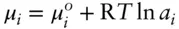
The “catch” on selecting a standard state for ƒ°, and hence for determining a iin eqn. 3.46, is that this state must be the same as the standard state for μ° . Thus, we need to bear in mind that standard states are implicit in the definition of activities, and that those standard states are tied to the standard-state chemical potential. Until the standard state is specified, activities have no meaning.
Comparing eqn. 3.46with 3.26 leads to:
(3.47) 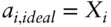
Thus, in ideal solutions, the activity is equal to the mole fraction.
Chemical potentials can be thought of as driving forces that determine the distribution of components between phases of variable composition in a system. Activities can be thought of as the effective concentration or the availability of components for reaction . In real solutions, it would be convenient to relate all nonideal thermodynamic parameters to the composition of the solution, because composition is generally readily and accurately measured. To relate activities to mole fractions, we define a new parameter, the rational activity coefficient , λ. The relationship is:
(3.48) 
The rational activity coefficient differs slightly in definition from the practical activity coefficient, γ, used in aqueous solutions. λ is defined in terms of mole fraction, whereas γ is variously defined in terms of moles of solute per moles of solvent, or more commonly, moles of solute per kg or liter of solution. Consider, for example, the activity of Na in an aqueous sodium chloride solution. For λ Na, X is computed as:
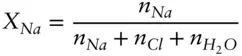
whereas for γ Na, X Nais:
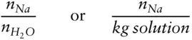
where n indicates moles of substance. γ is also used for other concentration units that we will introduce in section 3.7.
Example 3.2Using fugacity to calculate Gibbs free energy
The minerals brucite (Mg(OH) 2) and periclase (MgO) are related by the reaction:

Which side of this reaction represents the stable phase assemblage at 600°C and 200 MPa?
Answer: We learned how to solve this sort of problem in Chapter 2: the side with the lowest Gibbs free energy will be the stable assemblage. Hence, we need only to calculate Δ G rat 600°C and 200 MPa. To do so, we use eqn. 2.130:
(2.130) 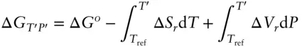
Our earlier examples dealt with solids, which are incompressible to a good approximation so we could simply treat Δ V ras independent of pressure. In that case, the solution to the first integral on the left was simply Δ V r( P′ – P ref). The reaction in this case, like most metamorphic reactions, involves H 2O, which is certainly not incompressible: its volume as steam or a supercritical fluid is very much a function of pressure. Let's isolate the difficulty by dividing Δ V rinto two parts: the volume change of reaction due to the solids, in this case the difference between molar volumes of periclase and brucite, and the volume change due to H 2O. We will denote the former as Δ V Sand assume that it is independent of pressure. The second integral in eqn. 2.132 then becomes:
(3.49) 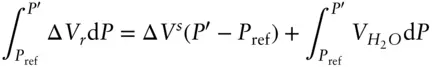
How do we solve the pressure integral above? One approach is to assume that H 2O is an ideal gas.
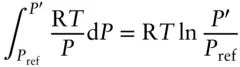
For an ideal gas:

so that the pressure integral becomes:
Steam is a very nonideal gas, so this approach would not yield a very accurate answer. The concept of fugacity provides us with an alternative solution. For a nonideal substance, fugacity bears the same relationship to volume as the pressure of an ideal gas. Hence, we may substitute fugacity for pressure so that the pressure integral in eqn. 2.130becomes:
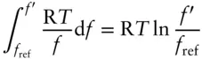
where we take the reference fugacity to be 0.1 MPa. Equation 3.49thus becomes:
(3.50) 
We can then compute fugacity using eqn. 3.44and the fugacity coefficients in Table 3.1.
Using the data in Table 2.2and solving the temperature integral in 2.130 as usual (eqn. 2.132), we calculate the Δ G T,Pis 3.29 kJ. As it is positive, the left side of the reaction, i.e., brucite, is stable.
The Δ S of this reaction is positive, however, implying that at some temperature, periclase plus water will eventually replace brucite. To calculate the actual temperature of the phase boundary requires a trial and error approach: for a given pressure, we must first guess a temperature, then look up a value of φ in Table 2.1(interpolating as necessary), and calculate Δ G r. Depending on our answer, we make a revised guess of T and repeat the process until Δ G is 0. Using a spreadsheet, however, this goes fairly quickly. Using this method, we calculate that brucite breaks down at 660°C at 200 MPa, in excellent agreement with experimental observations.
3.6.4 Excess functions
The ideal solution model provides a useful reference for solution behavior. Comparing real solutions with ideal ones leads to the concept of excess functions , for example:
(3.51) 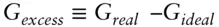
which can be resolved into contributions of excess enthalpy and entropy:
(3.52) 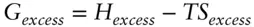
Интервал:
Закладка:
Похожие книги на «Geochemistry»
Представляем Вашему вниманию похожие книги на «Geochemistry» списком для выбора. Мы отобрали схожую по названию и смыслу литературу в надежде предоставить читателям больше вариантов отыскать новые, интересные, ещё непрочитанные произведения.


Обсуждение, отзывы о книге «Geochemistry» и просто собственные мнения читателей. Оставьте ваши комментарии, напишите, что Вы думаете о произведении, его смысле или главных героях. Укажите что конкретно понравилось, а что нет, и почему Вы так считаете.