Philippe J. S. De Brouwer - The Big R-Book

In the example about creating a factor-object for feedback one will have noticed that the plotfunction does show the labels in alphabetical order and not in an order that for us – humans – would be logical. It is possible to coerce a certain order in the labels by providing the levels – in the correct order – while creating the factor-object.

feedback <- c(‘Good’,‘Good’,‘Bad’,‘Average’,‘Bad’,‘Good’) factor_feedback <- factor(feedback, levels= c(“Bad”,“Average”,“Good”)) plot(factor_feedback)

In Figure 4.2on page 63 we notice that the order is now as desired (it is the order that we have provided via the attribute labelsin the function factor().

gl(n, k, length = n*k, labels = seq_len(n), ordered = FALSE) with

n: The number of levels

k: The number of replications (for each level)

length (optional): An integer giving the length of the result

labels (optional): A vector with the labels

ordered: A boolean variable indicating whether the results should be ordered.

gl()

gl(3,2,, c(“bad”,“average”,“good”),TRUE) ## [1] bad bad average average good good ## Levels: bad < average < good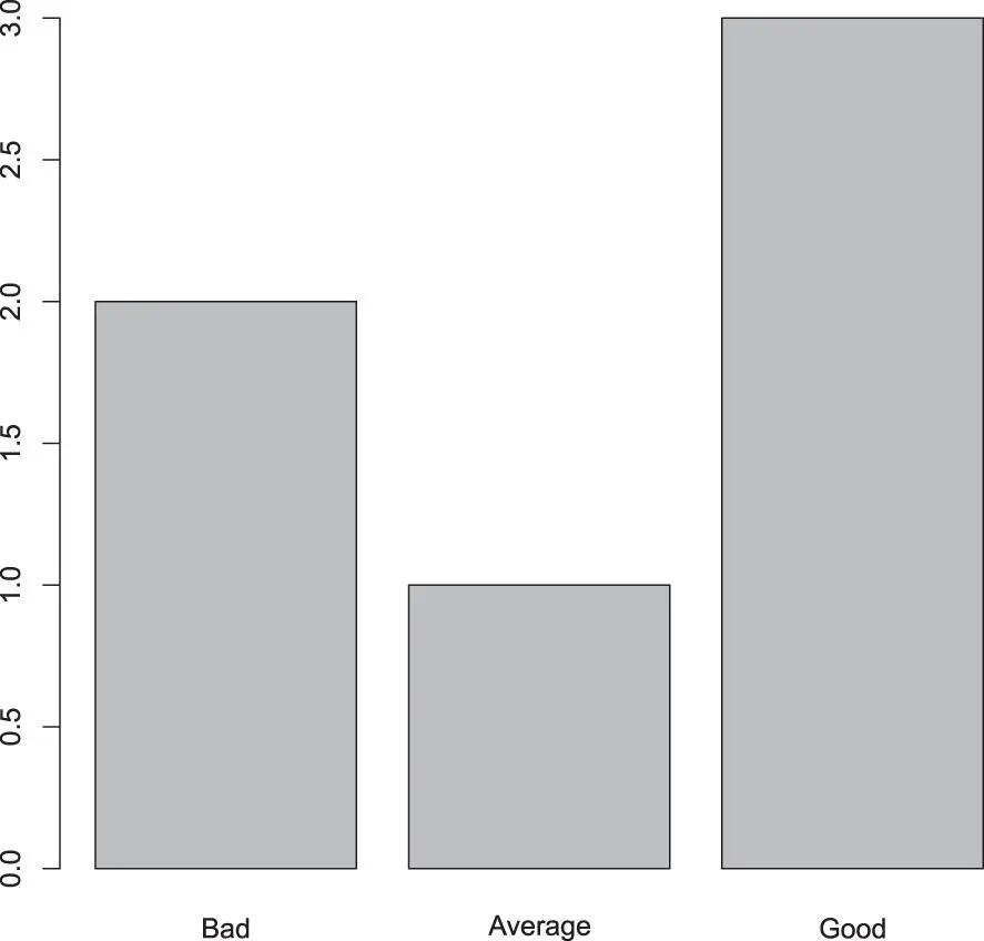

Figure 4.2 : The factor objects appear now in a logical order.

Use the dataset mtcars (from the library MASS) and explore the distribution of number of gears. Then explore the correlation between gears and transmission.

Then focus on the transmission and create a factor-object with the words “automatic” and “manual” instead of the numbers 0 and 1.

Use the ?mtcarsto find out the exact definition of the data.

mtcars

Use the dataset mtcars (fromthe libraryMASS) and explore the distribution of the horsepower (hp). How would you proceed to make a factoring (e.g. Low, Medium, High) for this attribute? Hint: Use the function cut().

cut()

Data frames are the prototype of all two-dimensional data (also known as “rectangular data”). For statistical analysis this is obviously an important data-type.

data frame

rectangular data

Data frames are very useful for statistical modelling; they are objects that contain data in a tabular way. Unlike a matrix in data frame each column can contain different types of data. For example, the first column can be factorial, the second logical, and the third numerical. It is a composite data type consisting of a list of vectors of equal length.

Data frames are created using the data.frame()function.

data.frame()

# Create the data frame.data_test <- data.frame( Name = c(“Piotr”, “Pawel”,“Paula”,“Lisa”,“Laura”), Gender = c(“Male”, “Male”,“Female”, “Female”,“Female”), Score = c(78,88,92,89,84), Age = c(42,38,26,30,35) ) print(data_test) ## Name Gender Score Age ## 1 Piotr Male 78 42 ## 2 Pawel Male 88 38 ## 3 Paula Female 92 26 ## 4 Lisa Female 89 30 ## 5 Laura Female 84 35 # The standard plot function on a data-frame (Figure 4.3) # with the pairs() function: plot(data_test)

pairs()

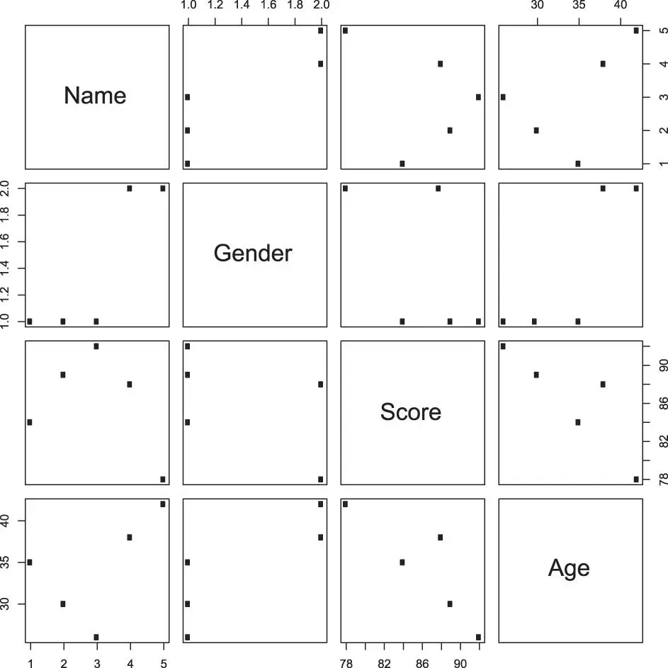
Figure 4.3 : The standard plot for a data frame in R shows each column printed in function of each other. This is useful to see correlations or how generally the data is structured.

Most data is rectangular, and in almost any analysis we will encounter data that is structured in a data frame. The following functions can be helpful to extract information from the data frame, investigate its structure and study the content.

summary()

head()

tail()

# Get the structure of the data frame: str(data_test) ## ‘data.frame’: 5 obs. of 4 variables: ## $ Name : Factor w/ 5 levels “Laura”,“Lisa”,..: 5 4 3 2 1 ## $ Gender: Factor w/ 2 levels “Female”,“Male”: 2 2 1 1 1 ## $ Score : num 78 88 92 89 84 ## $ Age : num 42 38 26 30 35 # Note that the names became factors (see warning below) # Get the summary of the data frame: summary(data_test) ## Name Gender Score Age ## Laura:1 Female:3 Min. :78.0 Min. :26.0 ## Lisa :1 Male :2 1st Qu.:84.0 1st Qu.:30.0 ## Paula:1 Median :88.0 Median :35.0 ## Pawel:1 Mean :86.2 Mean :34.2 ## Piotr:1 3rd Qu. :89.0 3rd Qu.:38.0 ## Max. :92.0 Max. :42.0 # Get the first rows: head(data_test) ## Name Gender Score Age ## 1 Piotr Male 78 42 ## 2 Pawel Male 88 38 ## 3 Paula Female 92 26 ## 4 Lisa Female 89 30 ## 5 Laura Female 84 35 # Get the last rows: tail(data_test) ## Name Gender Score Age ## 1 Piotr Male 78 42 ## 2 Pawel Male 88 38 ## 3 Paula Female 92 26 ## 4 Lisa Female 89 30 ## 5 Laura Female 84 35 # Extract the column 2 and 4 and keep all rowsdata_test.1 <-data_test[, c(2,4)] print(data_test.1) ## Gender Age ## 1 Male 42 ## 2 Male 38 ## 3 Female 26 ## 4 Female 30 ## 5 Female 35 # Extract columns by name and keep only selected rowsdata_test[ c(2 :4), c(2,4)] ## Gender Age ## 2 Male 38 ## 3 Female 26 ## 4 Female 30

The default behaviour of R is to convert strings to factors when a data.frame is created. Decades ago this was useful for performance reasons. Now, this is usually unwanted behaviour. a To avoid this put stringsAsFactors = FALSEin the data.frame()function.

d <- data.frame( Name = c(“Piotr”, “Pawel”,“Paula”,“Lisa”,“Laura”), Gender = c(“Male”, “Male”,“Female”, “Female”,“Female”), Score = c(78,88,92,89,84), Age = c(42,38,26,30,35), stringsAsFactors = FALSE ) d $Gender <- factor(d $Gender) # manually factorize gender str(d) ## ‘data.frame’: 5 obs. of 4 variables: ## $ Name : chr “Piotr” “Pawel” “Paula” “Lisa” … ## $ Gender: Factor w/ 2 levels “Female”,“Male”: 2 2 1 1 1 ## $ Score : num 78 88 92 89 84 ## $ Age : num 42 38 26 30 35