Philippe J. S. De Brouwer - The Big R-Book

While in general naming rows and/or columns is more relevant for datasets than matrices it is possible to work with matrices to store data if it only contains one type of variable.

row_names = c("row1", "row2", "row3", "row4") col_names = c("col1", "col2", "col3") M <- matrix( c(10 :21), nrow = 4, byrow = TRUE, dimnames = list(row_names, col_names)) print(M) ## col1 col2 col3 ## row1 10 11 12 ## row2 13 14 15 ## row3 16 17 18 ## row4 19 20 21

dimnames

Once thematrix exists, the columns and rows can be renamed with the functions colnames()and rownames()

colnames()

rownames()

colnames(M) <- c(‘C1’, ‘C2’, ‘C3’) rownames(M) <- c(‘R1’, ‘R2’, ‘R3’, ‘R4’) M ## C1 C2 C3 ## R1 10 11 12 ## R2 13 14 15 ## R3 16 17 18 ## R4 19 20 21

It might be obvious, that we can access one element of a matrix by using the row and column number. That is not all, R has a very flexible – but logical – model implemented. Let us consider a few examples that speak for themselves.

M <- matrix( c(10 :21), nrow = 4, byrow = TRUE) M ## [,1] [,2] [,3] ## [1,] 10 11 12 ## [2,] 13 14 15 ## [3,] 16 17 18 ## [4,] 19 20 21 # Access one element:M[1,2] ## [1] 11 # The second row:M[2,] ## [1] 13 14 15 # The second column:M[,2] ## [1] 11 14 17 20 # Row 1 and 3 only:M[ c(1, 3),] ## [,1] [,2] [,3] ## [1,] 10 11 12 ## [2,] 16 17 18 # Row 2 to 3 with column 3 to 1M[2 :3, 3 :1] ## [,1] [,2] [,3] ## [1,] 15 14 13 ## [2,] 18 17 16

Matrix arithmetic allows both base operators and specific matrix operations. The base operators operate always element per element.

Basic arithmetic on matrices works element by element:

M1 <- matrix( c(10 :21), nrow = 4, byrow = TRUE) M2 <- matrix( c( :11), nrow = 4, byrow = TRUE) M1 +M2 ## [,1] [,2] [,3] ## [1,] 10 12 14 ## [2,] 16 18 20 ## [3,] 22 24 26 ## [4,] 28 30 32 M1 *M2 ## [,1] [,2] [,3] ## [1,] 0 11 24 ## [2,] 39 56 75 ## [3,] 96 119 144 ## [4,] 171 200 231 M1 /M2 ## [,1] [,2] [,3] ## [1,] Inf 11.000000 6.000000 ## [2,] 4.333333 3.500000 3.000000 ## [3,] 2.666667 2.428571 2.250000 ## [4,] 2.111111 2.000000 1.909091

Write a function for the dot-product for matrices. Add also some security checks. Finally, compare your results with the “%*%-operator.”

dot-product

The dot-product is pre-defined via the %*%opeartor. Note that the function t()creates the transposed vector or matrix.

# Example of the dot-product:a <- c(1 :3) a %*%a ## [,1] ## [1,] 14 a %*% t(a) ## [,1] [,2] [,3] ## [1,] 1 2 3 ## [2,] 2 4 6 ## [3,] 3 6 9 t(a) %*%a ## [,1] ## [1,] 14 # Define A:A <- matrix( :8, nrow = 3, byrow = TRUE) # Test products:A %*%a ## [,1] ## [1,] 8 ## [2,] 26 ## [3,] 44 A %*% t(a) # this is bound to fail! ## Error in A %*% t(a): non-conformable argumentsA %*%A ## [,1] [,2] [,3] ## [1,] 15 18 21 ## [2,] 42 54 66 ## [3,] 69 90 111

There are also other operations possible on matrices. For example the quotient works as follows:

A %/%A ## [,1] [,2] [,3] ## [1,] NA 1 1 ## [2,] 1 1 1 ## [3,] 1 1 1

Note that matrices will accept both normal operators and specific matrix operators.

# Note the difference between the normal product:A *A ## [,1] [,2] [,3] ## [1,] 0 1 4 ## [2,] 9 16 25 ## [3,] 36 49 64 # and the matrix product %*%:A %*%A ## [,1] [,2] [,3] ## [1,] 15 18 21 ## [2,] 42 54 66 ## [3,] 69 90 111 # However, there is -of course- only one sum:A +A ## [,1] [,2] [,3] ## [1,] 0 2 4 ## [2,] 6 8 10 ## [3,] 12 14 16 # Note that the quotients yield almost the same:A %/%A ## [,1] [,2] [,3] ## [1,] NA 1 1 ## [2,] 1 1 1 ## [3,] 1 1 1 A /A ## [,1] [,2] [,3] ## [1,] NaN 1 1 ## [2,] 1 1 1 ## [3,] 1 1 1

The same hold for quotient and other operations.

Note that while exp ( A ), for example, is well defined for a matrix as the sum of the series:

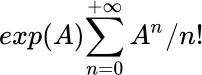
R will resort to calculating the exp () element by element!

Using the same matrix A as in the aforementioned code:

# This is the matrix A:A ## [,1] [,2] [,3] ## [1,] 0 1 2 ## [2,] 3 4 5 ## [3,] 6 7 8 # The exponential of A: exp(A) ## [,1] [,2] [,3] ## [1,] 1.00000 2.718282 7.389056 ## [2,] 20.08554 54.598150 148.413159 ## [3,] 403.42879 1096.633158 2980.957987

The same holds for all other functions of base R:

# The natural logarithm log(A) ## [,1] [,2] [,3] ## [1,] -Inf 0.000000 0.6931472 ## [2,] 1.098612 1.386294 1.6094379 ## [3,] 1.791759 1.945910 2.0794415 sin(A) ## [,1] [,2] [,3] ## [1,] 0.0000000 0.8414710 0.9092974 ## [2,] 0.1411200 -0.7568025 -0.9589243 ## [3,] -0.2794155 0.6569866 0.9893582

Note also that some operations will collapse the matrix to another (simpler) data type.

# Collapse to a vectore: colSums(A) ## [1] 9 12 15 rowSums(A) ## [1] 3 12 21 # Some functions aggregate the whole matrix to one scalar: mean(A) ## [1] 4 min(A) ## [1] 0

We already saw the function t()to transpose a matrix. There are a few others available in base R. For example, the function diag()diagonal matrix that is a subset of the matrix, det()caluclates the determinant, etc. The function solve()will solve the equation A %.% x = b, but when A is missing, it will assume the idenity vector and return the inverse of A .

diag()

solve()

M <- matrix( c(1,1,4,1,2,3,3,2,1), 3, 3) M ## [,1] [,2] [,3] ## [1,] 1 1 3 ## [2,] 1 2 2 ## [3,] 4 3 1 # The diagonal of M: diag(M) ## [1] 1 2 1 # Inverse: solve(M) ## [,1] [,2] [,3] ## [1,] 0.3333333 -0.66666667 0.33333333 ## [2,] -0.5833333 0.91666667 -0.08333333 ## [3,] 0.4166667 -0.08333333 -0.08333333 # Determinant: det(M) ## [1] -12 # The QR composition:QR_M <- qr(M) QR_M $rank ## [1] 3 # Number of rows and columns: nrow(M) ## [1] 3 ncol(M) ## [1] 3 # Sums of rows and columns: colSums(M) ## [1] 6 6 6 s rowSums(M) ## [1] 5 5 8 # Means of rows, columns, and matrix: colMeans(M) ## [1] 2 2 2 rowMeans(M) ## [1] 1.666667 1.666667 2.666667 mean(M) ## [1] 2 # Horizontal and vertical concatenation: rbind(M, M) ## [,1] [,2] [,3] ## [1,] 1 1 3 ## [2,] 1 2 2 ## [3,] 4 3 1 ## [4,] 1 1 3 ## [5,] 1 2 2 ## [6,] 4 3 1 cbind(M, M) ## [,1] [,2] [,3] [,4] [,5] [,6] ## [1,] 1 1 3 1 1 3 ## [2,] 1 2 2 1 2 2 ## [3,] 4 3 1 4 3 1