Michael Begon - Ecology

(5.27)

where a is a constant. Similarly, we expect mean plant weight, P , to be related to D by:

(5.28)

where b is also a constant. Putting Equations 5.26– 5.28together, we obtain:

(5.29)

This is structurally equivalent to the −3/2 power relationship in Equation 5.23, with the intercept constant, c , given by b(L/a) 3/2.

It is apparent, therefore, why thinning lines might generally be expected to have slopes of approximately −3/2. Moreover, if the relationships in Equations 5.27and 5.28were roughly the same for all plant species, and if all plants supported roughly the same leaf area per unit area of ground ( L ), then the constant c would be approximately the same for all species. On the other hand, suppose that L is not quite the same for all species, or that the powers in Equations 5.27and 5.28are not exactly 2 or 3, or that the constants in these equations ( a and b ) either vary between species or are not actually constants at all. Thinning lines will then have slopes that depart from −3/2, and slopes and intercepts that vary from species to species. It is easy to see why, according to the areal argument, there is a broad similarity in the behaviour of different species, but also why, on closer examination, there are likely to be variations between species and no such thing as a single, ‘ideal’ thinning line.

complications of the areal argument

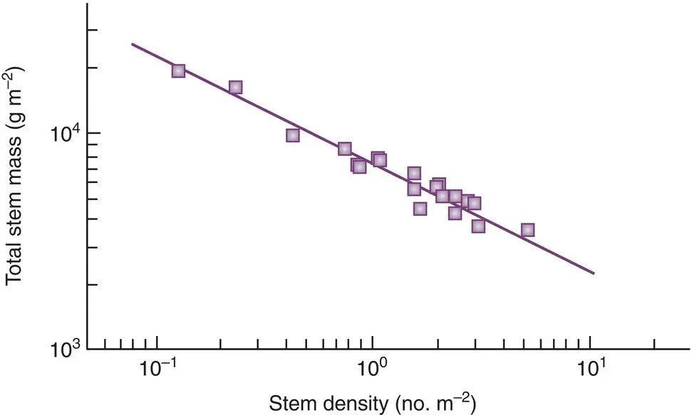
Furthermore, contrary to the simple areal argument, the yield–density relationship in a growing cohort need not depend only on the numbers that die and the way the survivors grow. We have seen (see Section 5.8) that competition is frequently highly asymmetric. If those that die in a cohort are predominantly the very smallest individuals, then density ( individuals per unit area) will decline more rapidly as the cohort grows than it would otherwise do. It seems possible, too, to use departures from the assumptions built into Equations 5.26– 5.29to explain at least some of the variations from a ‘general’ −3/2 rule. We see this in a study by Osawa and Allen (1993), who estimated a number of the parameters in these equations from data on the growth of individual plants from two species: mountain beech ( Nothofagus solandri ) and red pine ( Pinus densiflora ). They estimated, for instance, that the exponents in Equations 5.27and 5.28were not 2 and 3, but 2.08 and 2.19 for mountain beech, and 1.63 and 2.41 for red pine. These suggest thinning slopes of −1.05 in the first case and −1.48 in the second, which compare quite remarkably well with the slopes that they observed: −1.06 and −1.48 ( Figure 5.38). The similarities between the estimates and observations for the intercept constants were equally impressive. These results show, therefore, that thinning lines with slopes other than −3/2 can occur, but can be explicable in terms of the detailed biology of the species concerned. They also show that even when slopes of −3/2 do occur, they may do so, as with red pine, for the ‘wrong’ reason (−2.41/1.63 rather than −3/2).

Figure 5.38 The species boundary line for populations of red pine, Pinus densiflora , from northern Japan (slope = −1.48).

Source : After Osawa & Allen (1993).

self‐thinning in sessile animals

Animals must also ‘self‐thin’, insofar as growing individuals within a cohort increasingly compete with one another and reduce their own density. And in the case of some sessile, aquatic animals, we can think of them, like plants, as being reliant on a resource falling from above (typically food particles in the water) and therefore needing to pack ‘volumes’ beneath an approximately constant area. It is striking, therefore, that in studies on rocky‐shore invertebrates, mussels have been found to follow a thinning line with a slope of −1.4, barnacles a line with a slope of −1.6 (Hughes & Griffiths, 1988), and gregarious tunicates a slope of −1.5 (Guiñez & Castilla, 2001). There is, however, nothing linking all animals quite like the shared need for light interception that links all plants.

This need to include all types of organisms in considerations of self‐thinning is reflected in studies seeking alternative explanations for the underlying trend itself. Most notably, Enquist et al . (1998) made use of the much more general model of West et al . (1997) that we discussed in Chapter 3, which considered the most effective architectural designs of organisms. We saw there that the rate of resource use per individual, u , or more simply their metabolic rate, should be related to mean organism body mass, M , according to the equation:

(5.30)

where a is a constant and the value ¾ is the ‘allometric exponent’.

−4/3 or −3/2?

They then argued that we can expect organisms to have evolved to make full use of the resources available, and so if S is the rate of resource supply per unit area and N maxthe maximum density of organisms possible at this supply rate, then:

(5.31)

or, from Equation 5.30:

(5.32)

But if the organisms have arrived at an equilibrium with the rate of resource supply, then S should itself be constant. Hence:

(5.33)

where c is another constant. In short, the expected slope of a population boundary on this argument is −4/3 rather than −3/2. Similarly, the figure in biomass–density relationships ( equations 5.24and 5.25) would be −1/3 rather than −1/2.

Enquist and colleagues themselves considered the available data to be more supportive of their prediction of a slope of −4/3 than the more conventional −3/2, though this had not been the conclusion drawn from previous data surveys. Indeed, as we saw in Chapter 3, the idea of ¾ being a consistent or universal allometric exponent, and a slope of −4/3 therefore being expected, has itself been called increasingly into question (e.g. Glazier, 2005). Nonetheless, Begon et al . (1986) had found a mean value of −1.29 (close to a value of −4/3) for self‐thinning in experimental cohorts of grasshoppers, and Elliott (1993) a value of −1.35 for a population of sea trout, Salmo trutta , in the English Lake District. On the other hand, studies on house crickets, Acheta domesticus , have shown that the allometric exponent in in their case is not ¾ but 0.9 (Jonsson, 2017), and the estimated slope of their self‐thinning line −1.11 (the exact reciprocal of the allometric exponent; Figure 5.39a).