Matthew B. Hamilton - Population Genetics

(2.19)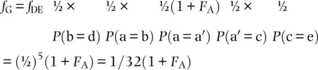

since independent probabilities can be multiplied to find the total probability of an event. This is equivalent to the average relatedness among half‐cousins. In general, for pedigrees, f = (½) i(1 + F A) where A is the common ancestor and i is the number of paths or individuals over which alleles are transmitted. By writing down the chain of individuals and counting the individuals along paths of inheritance, we can determine the probability that a sample of two alleles, one from each individual, would exhibit both alleles identical by descent. That method gives GDBACEG or five ancestors for , yielding a result identical to Eq. 2.19.

We can use the method of tracing paths between ancestors to determine the coancestry coefficient, often symbolized by Θ,for any type of relationship. The pedigree in Figure 2.16provides a set of examples of close relatives where we can determine the coancestry coefficient using paths of inheritance. In general, coefficients of coancestry for two individuals A and B can be determined using

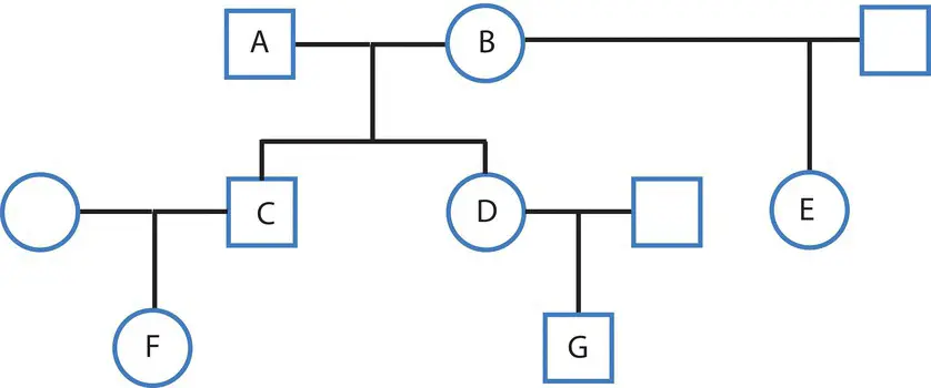
Figure 2.16 A pedigree showing first (A and C are parent and offspring, C and D are full siblings), second (A and B are the grandparents of F and G, D, and E are half siblings), and third (F and G are cousins) degree relatives. The coancestry coefficient gives the probability that an allele sampled from each of two related individuals is identical by descent, defining the degree of relatedness.

(2.20)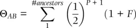

where P is the number of ancestor–descendant paths connecting A and B, and F is the homozygote excess or deficit of the ancestor (Wright 1922; Thompson 1988). The inbreeding coefficientof an individual, or the probability of an individual inheriting two copies of the same allele, is a function of the coancestry of its parents. One example is the coancestry between one parent and an offspring, such as individuals A and C in Figure 2.16. There is one ancestor–descendant link between A and C, so the coancestry coefficient is

(2.21)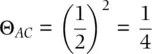

assuming that the parent A has F = 0. For the parent, the chance of sampling the allele that was transmitted to the offspring is ½. For the offspring too, the chance of sampling the allele inherited from that parent is ½. When combined, the chance of sampling the one allele that is identical by descent (IBD) between parents and offspring is (1/2) 2= 1/4. When considering both alleles in the offspring, one of them is IBD to one parent, so a parent and an offspring are ¼ + ¼ = ½ related.

The coancestry coefficient for full siblings, such as individuals C and D in Figure 2.16, is a case where individuals share two parents in common and therefore have two common ancestors to account for. Counting the paths C–A–D and C–B–D, we obtain

(2.22)

The chance that a given allele was transmitted from one parent to one offspring is ½, with a probability of (1/2) 2= ¼ of both full siblings inheriting the same allele from one parent. Because C and D share both parents and can inherit alleles identical by descent from both, we add the coancestries of each allele to give a relatedness of 1/4 + 1/4 = ½.

The coancestry coefficients for self‐fertilization and for full siblings explain the pattern of decreasing heterozygosity and increasing fixation indices over generations seen in Figure 2.13. For self‐fertilization, each generation has a coancestry coefficient of ½ when a self‐fertilized parent descended from unrelated individuals, making the fixation index equal to ½ after one generation of selfing. For a second generation of self‐fertilization, the coancestry coefficient remains ½ but now the parent has a higher probability of being homozygous because of the first generation of selfing. This makes the second‐generation fixation index F 3= ½(1 + ½) = 3/4.

In the case of full siblings, the recursion equation is F t + 2= ¼(1 + 2 F t + 1+ F t). For full siblings, the coancestry coefficient is ¼ when their parents have no history of consanguineous mating among their ancestors, resulting in F 2= ¼. Taking two individuals from the second generation of full sibling mating as parents means that they each have a higher probability of being homozygous that is added to the constant ¼ probability of coancestry for full siblings. This gives a fixation index after three generations of full sibling mating of F 3= ¼(1 + 2[¼] + 0) = 3/8 (it is not until the fourth generation that the grandparents in generation t have a fixation index greater than zero).

It is useful to determine the coancestry coefficient for a specific set of relatives or pedigree as well as the change in the fixation index over generations for mating systems, especially in quantitative genetics. With the recent ability to obtain genome‐scale DNA sequences of numerous individuals, it is now possible to estimate coancestry directly from observed DNA polymorphism. Direct estimation of shared DNA using sequences highlights that traditional coancestry coefficients obtained from pedigrees are an average for a large sample of individuals and there can be substantial variation around these averages in the DNA‐level relatedness of an observed set of individuals (Ackerman et al. 2017). The general point is to understand that mating among relatives as a process that increases autozygosity in a population. When individuals have common relatives, the chance that they share alleles identical by descent is increased as is the chance that the genotype of one individual is homozygous.

The departure from Hardy–Weinberg expected genotype frequencies, the coancestry coefficient, the autozygosity, and the fixation index are interrelated. Another way of stating the results that were developed in Figure 2.12is that F measures the degree to which Hardy–Weinberg genotype frequencies are not met due to departure from purely random union of alleles in diploid genotypes as expressed by f . To see this, imagine starting with a one locus with two alleles in a population at Hardy–Weinberg expected genotype frequencies with F equal zero. The expected frequencies of the three genotypes in progeny could be expressed as

Genetic genealogy is the use of DNA testing to augment historical records with the goal of identifying ancestors and descendants. The approach is to use autosomal, Y‐chromosome, and mitochondrial DNA genetic markers to locate relatives based on observed sharing of alleles and haplotypes. With enough genetic loci, even distant relatives who have small coancestry coefficients can be identified if their genotypes are available for comparison. Genetic profile data has been collected for millions of individuals who have participated in direct‐to‐consumer DNA testing. Applications include reconstruction of family histories, identification of ancestral population origins, and identifying the biological parents of adoptees.