Matthew B. Hamilton - Population Genetics
Здесь есть возможность читать онлайн «Matthew B. Hamilton - Population Genetics» — ознакомительный отрывок электронной книги совершенно бесплатно, а после прочтения отрывка купить полную версию. В некоторых случаях можно слушать аудио, скачать через торрент в формате fb2 и присутствует краткое содержание. Жанр: unrecognised, на английском языке. Описание произведения, (предисловие) а так же отзывы посетителей доступны на портале библиотеки ЛибКат.
- Название:Population Genetics
- Автор:
- Жанр:
- Год:неизвестен
- ISBN:нет данных
- Рейтинг книги:4 / 5. Голосов: 1
-
Избранное:Добавить в избранное
- Отзывы:
-
Ваша оценка:
Population Genetics: краткое содержание, описание и аннотация
Предлагаем к чтению аннотацию, описание, краткое содержание или предисловие (зависит от того, что написал сам автор книги «Population Genetics»). Если вы не нашли необходимую информацию о книге — напишите в комментариях, мы постараемся отыскать её.
is the classic, accessible introduction to the concepts of population genetics. Combining traditional conceptual approaches with classical hypotheses and debates, the book equips students to understand a wide array of empirical studies that are based on the first principles of population genetics.
Featuring a highly accessible introduction to coalescent theory, as well as covering the major conceptual advances in population genetics of the last two decades, the second edition now also includes end of chapter problem sets and revised coverage of recombination in the coalescent model, metapopulation extinction and recolonization, and the fixation index.
Population Genetics — читать онлайн ознакомительный отрывок
Ниже представлен текст книги, разбитый по страницам. Система сохранения места последней прочитанной страницы, позволяет с удобством читать онлайн бесплатно книгу «Population Genetics», без необходимости каждый раз заново искать на чём Вы остановились. Поставьте закладку, и сможете в любой момент перейти на страницу, на которой закончили чтение.
Интервал:
Закладка:
Product rule: The probability of two (or more) independent events occurring simultaneously is the product of their individual probabilities.
Now, we can return to the question of whether two unrelated individuals are likely to share an identical three‐locus DNA profile by chance. One out of every 20 408 Caucasian Americans is expected to have the genotype in Table 2.2. Although the three‐locus DNA profile is considerably less frequent than a genotype for a single locus, it still does not approach a unique, individual identifier. Therefore, there is a finite chance that a suspect will match an evidence DNA profile by chance alone. Such DNA profile matches, or “inclusions,” require additional evidence to ascertain guilt or innocence. In fact, the term prosecutor's fallacy was coined to describe failure to recognize the difference between a DNA match and guilt (for example, a person can be present at a location and not involved in a crime). Only when DNA profiles do not match, called an “exclusion,” can a suspect be unambiguously and absolutely ruled out as the source of a biological sample at a crime scene.
Current forensic DNA profiles use 10–13 loci to estimate expected genotype frequencies. Problem 2.1 gives a 10‐locus genotype for the same individual in Table 2.2, allowing you to calculate the odds ratio for a realistic example. In Chapter 4, we will reconsider the expected frequency of a DNA profile with the added complication of allele frequency differentiation among human racial groups.
Problem box 2.1 The expected genotype frequency for a DNA profile
Calculate the expected genotype frequency and odds ratio for the 10‐locus DNA profile below. Allele frequencies are given in Table 2.3.
| D3S1358 | 17, 18 |
| vWA | 17, 17 |
| FGA | 24, 25 |
| Amelogenin | X, Y |
| D8S1179 | 13, 14 |
| D21S11 | 29, 30 |
| D18S51 | 18, 18 |
| D5S818 | 12, 13 |
| D13S317 | 9, 12 |
| D7S820 | 11, 12 |
What does the amelogenin locus tell us and how did you assign an expected frequency to the observed genotype? Is it likely that two unrelated individuals would share this 10‐locus genotype by chance? For this genotype, would a match between a crime scene sample and a suspect be convincing evidence that the person was present at the crime scene?
Testing Hardy–Weinberg expected genotype frequencies
A common use of Hardy–Weinberg expectations is to test for deviations from its null model. Populations with genotype frequencies that do not fit Hardy–Weinberg expectations are evidence that one or more of the evolutionary processes embodied in the assumptions of Hardy–Weinberg are acting to determine genotype frequencies. Our null hypothesis is that genotype frequencies meet Hardy–Weinberg expectations within some degree of estimation error. Genotype frequencies that are not close to Hardy–Weinberg expectations allow us to reject this null hypothesis. The processes in the list of assumptions then become possible alternative hypotheses to explain observed genotype frequencies. In this section, we will work through a hypothesis test for Hardy–Weinberg equilibrium.
The first example uses observed genotypes for the MN blood group, a single locus in humans that has two alleles ( Table 2.4). First, we need to estimate the frequency of the M allele, using the notation that the estimated frequency of M is  and the frequency of N is
  . Note that the “hat” superscripts indicate that these are allele frequency estimates (see Chapter 1). The total number of alleles is 2 N given a sample of N diploid individuals. We can then count up all of the alleles of one type to estimate the frequency of that allele.
(2.5) 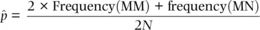
(2.6) 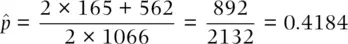
Since  , we can estimate the frequency of the N allele by subtraction as
  .
.
Using these allele frequencies allows calculation of the Hardy–Weinberg expected genotype frequency and number of individuals with each genotype, as shown in Table 2.4. In Table 2.4, we can see that the match between the observed and expected is not perfect, but we need some method to ask whether the difference is actually large enough to conclude that Hardy–Weinberg equilibrium does not hold in the sample of 1066 genotypes. Remember that any allele frequency estimate  could differ slightly from the true parameter ( p ) due to chance events as well as due to random sampling in the group of genotypes used to estimate the allele frequencies. Asking whether genotypes are in Hardy–Weinberg proportions is actually the same as asking whether a coin is “fair.” With a fair coin, we expect one‐half heads and one‐half tails if we flip it a large number of times. But even with a fair coin, we can get something other than exactly 50 : 50 even if the sample size is large. We would consider a coin fair if in 1000 flips it produced 510 heads and 490 tails. However, the hypothesis that a coin is fair would be in doubt if we observed 250 heads and 750 tails given that we expect 500 of each.
Box 2.1DNA profiling
The loci used for human DNA profiling are a general class of DNA sequence marker known as simple tandem repeat (STR), simple sequence repeat (SSR), or microsatellite loci. These loci feature tandemly repeated DNA sequences of one to six base pairs (bp) and often exhibit many alleles per locus and high levels of heterozygosity. Allelic states are simply the number of repeats present at the locus, which can be determined by electrophoresis of polymerase chain reaction (PCR) amplified DNA fragments. STR loci used in human DNA profiling generally exhibit Hardy–Weinberg expected genotype frequencies; there is evidence that the genotypes are selectively “neutral” (e.g. not affected by natural selection), and the loci meet the other assumptions of Hardy–Weinberg. STR loci are employed widely in population genetic studies and in genetic mapping (see reviews by Goldstein and Pollock 1997; McDonald and Potts 1997).
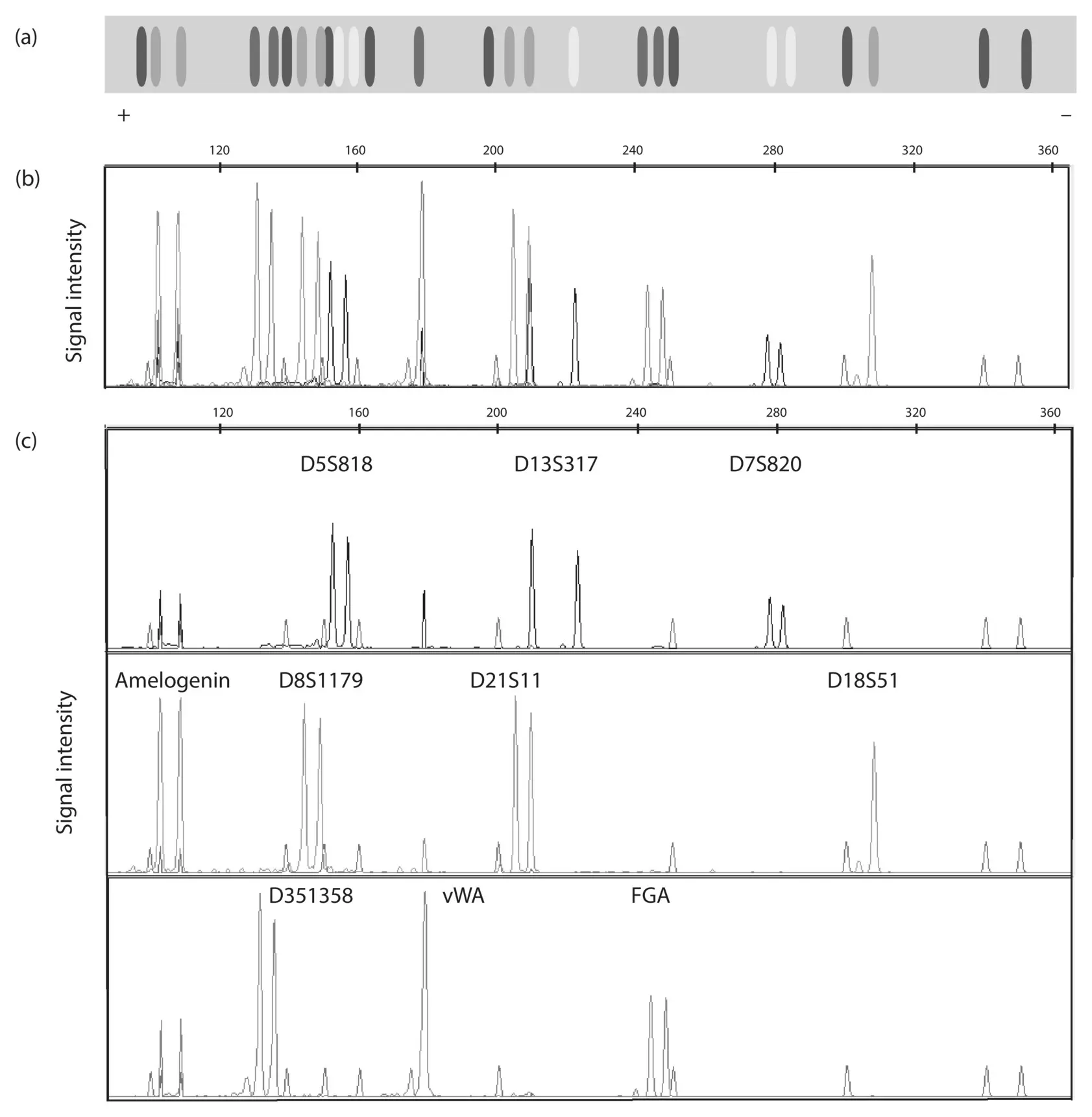
Figure 2.8 The original data for the DNA profile given in Table 2.2and Problem Box 2.1obtained by capillary electrophoresis. The PCR oligonucleotide primers used to amplify each locus are labeled with a molecule that emits blue, green, or yellow light when exposed to laser light. Thus, the DNA fragments for each locus are identified by their label color as well as their size range in base pairs. Panel A shows a simulation of the DNA profile as it would appear on an electrophoretic gel (+ indicates the anode side). Blue, green, and yellow label the 10 DNA profiling loci, shown here in grayscale. The red DNA fragments are size standards with a known molecular weight used to estimate the size in base pairs of the other DNA fragments in the profile. Panel B shows the DNA profile for all loci and the size standard DNA fragments as a graph of color signal intensity by size of DNA fragment in base pairs. Panel C shows a simpler view of trace data for each label color independently with the individual loci labeled above the trace peaks. A few shorter peaks are visible in the yellow, green, and blue traces of Panel C that are not labeled as loci. These artifacts, called “pull up” peaks, are caused by intense signal from a locus labeled with another color (e.g. the yellow and blue peaks in the location of the green labeled amelogenin locus ). A full color version of this figure is available on the textbook website.
Читать дальшеИнтервал:
Закладка:
Похожие книги на «Population Genetics»
Представляем Вашему вниманию похожие книги на «Population Genetics» списком для выбора. Мы отобрали схожую по названию и смыслу литературу в надежде предоставить читателям больше вариантов отыскать новые, интересные, ещё непрочитанные произведения.


Обсуждение, отзывы о книге «Population Genetics» и просто собственные мнения читателей. Оставьте ваши комментарии, напишите, что Вы думаете о произведении, его смысле или главных героях. Укажите что конкретно понравилось, а что нет, и почему Вы так считаете.