Matthew B. Hamilton - Population Genetics
Здесь есть возможность читать онлайн «Matthew B. Hamilton - Population Genetics» — ознакомительный отрывок электронной книги совершенно бесплатно, а после прочтения отрывка купить полную версию. В некоторых случаях можно слушать аудио, скачать через торрент в формате fb2 и присутствует краткое содержание. Жанр: unrecognised, на английском языке. Описание произведения, (предисловие) а так же отзывы посетителей доступны на портале библиотеки ЛибКат.
- Название:Population Genetics
- Автор:
- Жанр:
- Год:неизвестен
- ISBN:нет данных
- Рейтинг книги:4 / 5. Голосов: 1
-
Избранное:Добавить в избранное
- Отзывы:
-
Ваша оценка:
Population Genetics: краткое содержание, описание и аннотация
Предлагаем к чтению аннотацию, описание, краткое содержание или предисловие (зависит от того, что написал сам автор книги «Population Genetics»). Если вы не нашли необходимую информацию о книге — напишите в комментариях, мы постараемся отыскать её.
is the classic, accessible introduction to the concepts of population genetics. Combining traditional conceptual approaches with classical hypotheses and debates, the book equips students to understand a wide array of empirical studies that are based on the first principles of population genetics.
Featuring a highly accessible introduction to coalescent theory, as well as covering the major conceptual advances in population genetics of the last two decades, the second edition now also includes end of chapter problem sets and revised coverage of recombination in the coalescent model, metapopulation extinction and recolonization, and the fixation index.
Population Genetics — читать онлайн ознакомительный отрывок
Ниже представлен текст книги, разбитый по страницам. Система сохранения места последней прочитанной страницы, позволяет с удобством читать онлайн бесплатно книгу «Population Genetics», без необходимости каждый раз заново искать на чём Вы остановились. Поставьте закладку, и сможете в любой момент перейти на страницу, на которой закончили чтение.
Интервал:
Закладка:
The columns in the offspring genotype frequency table are the basis of the final step. The sum of each column gives the total frequencies of each progeny genotype expected in generation t + 1. Let's take the sum of each column, again expressed in the currency of genotype frequencies, and then simplify the algebra to see whether Hardy and Weinberg were correct.
(2.4) 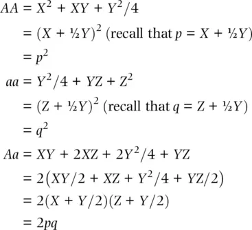
So, we have proved that progeny genotype and allele frequencies are identical to parental genotype and allele frequencies over one generation or that f(A) t= f(A) t + 1. The major conclusion here is that genotype frequencies remain constant over generations as long as the assumptions of Hardy–Weinberg are met . In fact, we have just proved that under Mendelian heredity, genotype and allele frequencies should not change over time unless one or more of our assumptions is not met. This simple model of expected genotype frequencies has profound conclusions. In fact, Hardy–Weinberg expected genotype frequencies serve as one of the most basic tools to test for the action of biological processes that alter genotype and allele frequencies.
You might wonder whether Hardy–Weinberg applies to loci with more than two alleles. For the last point in this section, let's explore that question. With three alleles at one locus (allele frequencies symbolized by p , q , and r ), Hardy–Weinberg expected genotype frequencies are p 2+ q 2+ r 2+ 2 pq + 2 pr + 2 qr = 1. These genotype frequencies are obtained by expanding ( p + q + r ) 2, a method that can be applied to any number of alleles at one locus. In general, expanding the squared sum of the allele frequencies will show:
the frequency of any homozygous genotype is the squared frequency of the single allele that composes the genotype ([allele frequency]2);
the frequency of any heterozygous genotype is twice the product of the two allele frequencies that comprise the genotype (2[allele 1 frequency][allele 2 frequency]), and
there are as many homozygous genotypes as there are alleles and heterozygous genotypes where N is the number of alleles.
Do you think it would be possible to prove Hardy–Weinberg for more than two alleles at one locus? The answer is absolutely, yes. This would just require constructing larger versions of the parental genotype mating table and expected offspring frequency table as we did for two alleles at one locus.
2.4 Applications of Hardy–Weinberg
Estimate the frequency of an observed genotype in a forensic DNA typing case.
Test the null hypothesis that observed and expected genotype frequencies are identical.
Use Hardy–Weinberg to compare two genetic models for observed phenotypes.
In the previous two sections, we established the Hardy–Weinberg expectations for genotype frequencies. In this section, we will examine three ways that expected genotype frequencies are employed in practice. The goal of this section is to become familiar with realistic applications as well as hypothesis tests that compare observed and Hardy–Weinberg expected genotype frequencies. In this process, we will also look at a specific method to account for sampling error (see Appendix).
Forensic DNA profiling
Our first application of Hardy–Weinberg can be found in newspapers on a regular basis and commonly dramatized on television. A terrible crime has been committed. Left at the crime scene was a biological sample that law enforcement authorities use to obtain a multilocus genotype or DNA profile. A suspect in the crime has been identified and subpoenaed to provide a tissue sample for DNA profiling. The DNA profile from the suspect and from the crime scene are identical. The DNA profile is shown in Table 2.2. Should we conclude that the suspect left the biological sample found at the crime scene?
To answer this critical question, we will employ Hardy–Weinberg to predict the expected frequency of the DNA profile or genotype. Just because two DNA profiles match, there is not necessarily strong evidence that the individual who left the evidence DNA and the suspect are the same person. It is possible that there are actually two or more people with identical DNA profiles. Hardy–Weinberg and Mendel's second law will serve as the bases for us to estimate just how frequently a given DNA profile should be observed. Then, we can determine whether two unrelated individuals sharing an identical DNA profile is a likely occurrence.
Table 2.2 An example DNA profile for three STR (“simple tandem repeat”) loci commonly used in human forensic cases. Locus names refer to the human chromosome (e.g. D3 = third chromosome) and chromosome region where the SRT locus is found. The allele states are the numbers of repeats at that locus (see Box 2.1).
| Locus | D3S1358 | D21S11 | D18S51 |
|---|---|---|---|
| Genotype | 17, 18 | 29, 30 | 18, 18 |
To determine the expected frequency of a one‐locus genotype, we employ the Hardy–Weinberg Eq. (2.1). In doing so, we are implicitly accepting that all of the assumptions of Hardy–Weinberg are approximately met. If these assumptions were not met, then the Hardy–Weinberg equation would not provide an accurate expectation for the genotype frequencies! To determine the frequency of the three‐locus genotype in Table 2.2, we need allele frequencies for those loci, which are found in Table 2.3. Starting with the locus D3S1358, we see in Table 2.3that the 17‐repeat allele has a frequency of 0.2118 and the 18‐repeat allele a frequency of 0.1626. Then, using Hardy–Weinberg, the 17, 18 genotype has an expected frequency of 2(0.2118)(0.1626) = 0.0689 or 6.89%. For the two other loci in the DNA profile of Table 2.2, we carry out the same steps.
| D21S11 | 29‐Repeat allele frequency = 0.1811 |
| 30‐Repeat allele frequency = 0.2321 | |
| Genotype frequency = 2(0.1811)(0.2321) = 0.0841 or 8.41% | |
| D18S51 | 18‐Repeat allele frequency = 0.0918 |
| Genotype frequency = (0.0918) 2= 0.0084 or 0.84% |
The genotype for each locus has a relatively large chance of being observed in a population. For example, a little less than 1% of Caucasian U.S. citizens (or about 1 in 119) are expected to be homozygous for the 18‐repeat allele at locus D18S51. Therefore, a match between evidence and suspect DNA profiles homozygous for the 18 repeat at that locus would not be strong evidence that the samples came from the same individual.
Table 2.3 Allele frequencies for nine STR loci commonly used in forensic cases estimated from 196 US Caucasians sampled randomly with respect to geographic location. The allele states are the numbers of repeats at that locus (see Box 2.1). Allele frequencies (Freq) are as reported in Budowle et al. (2001). Table 1 from FBI sample population.
| D3S1358 | vWA | D21S11 | D18S51 | D13S317 | |||||
|---|---|---|---|---|---|---|---|---|---|
| Allele | Freq | Allele | Freq | Allele | Freq | Allele | Freq | Allele | Freq |
| 12 | 0.0000 | 13 | 0.0051 | 27 | 0.0459 | <11 | 0.0128 | 8 | 0.0995 |
| 13 | 0.0025 | 14 | 0.1020 | 28 | 0.1658 | 11 | 0.0128 | 9 | 0.0765 |
| 14 | 0.1404 | 15 | 0.1122 | 29 | 0.1811 | 12 | 0.1276 | 10 | 0.0510 |
| 15 | 0.2463 | 16 | 0.2015 | 30 | 0.2321 | 13 | 0.1224 | 11 | 0.3189 |
| 16 | 0.2315 | 17 | 0.2628 | 30.2 | 0.0383 | 14 | 0.1735 | 12 | 0.3087 |
| 17 | 0.2118 | 18 | 0.2219 | 31 | 0.0714 | 15 | 0.1276 | 13 | 0.1097 |
| 18 | 0.1626 | 19 | 0.0842 | 31.2 | 0.0995 | 16 | 0.1071 | 14 | 0.0357 |
| 19 | 0.0049 | 20 | 0.0102 | 32 | 0.0153 | 17 | 0.1556 | ||
| 32.2 | 0.1122 | 18 | 0.0918 | ||||||
| 33.2 | 0.0306 | 19 | 0.0357 | ||||||
| 35.2 | 0.0026 | 20 | 0.0255 | ||||||
| 21 | 0.0051 | ||||||||
| 22 | 0.0026 | ||||||||
| FGA | D8S1179 | D5S818 | D7S820 | ||||||
| Allele | freq | Allele | freq | Allele | freq | Allele | Freq | ||
| 18 | 0.0306 | <9 | 0.0179 | 9 | 0.0308 | 6 | 0.0025 | ||
| 19 | 0.0561 | 9 | 0.1020 | 10 | 0.0487 | 7 | 0.0172 | ||
| 20 | 0.1454 | 10 | 0.1020 | 11 | 0.4103 | 8 | 0.1626 | ||
| 20.2 | 0.0026 | 11 | 0.0587 | 12 | 0.3538 | 9 | 0.1478 | ||
| 21 | 0.1735 | 12 | 0.1454 | 13 | 0.1462 | 10 | 0.2906 | ||
| 22 | 0.1888 | 13 | 0.3393 | 14 | 0.0077 | 11 | 0.2020 | ||
| 22.2 | 0.0102 | 14 | 0.2015 | 15 | 0.0026 | 12 | 0.1404 | ||
| 23 | 0.1582 | 15 | 0.1097 | 13 | 0.0296 | ||||
| 24 | 0.1378 | 16 | 0.0128 | 14 | 0.0074 | ||||
| 25 | 0.0689 | 17 | 0.0026 | ||||||
| 26 | 0.0179 | ||||||||
| 27 | 0.0102 |
Fortunately, we can combine the information from all three loci. To do this, we use the product rule, which states that the probability of observing multiple independent events is just the product of each individual event. We already used the product rule in the last section to calculate the expected frequency of each genotype under Hardy–Weinberg by treating each allele as an independent probability. Now, we just extend the product rule to cover multiple genotypes, under the assumption that each of the loci is independent by Mendel's second law (the assumption is justified here since each of the loci is on a separate chromosome). The expected frequency of the three‐locus genotype (sometimes called the probability of identity ) is then 0.0689 × 0.0841 × 0.0084 = 0.000049 or 0.0049%. Another way to express this probability is as an odds ratio, or the reciprocal of the probability (an approximation that holds when the probability is very small). Here, the odds ratio is 1/0.000049 = 20 408, meaning that we would expect to observe the three locus DNA profile once in 20 408 Caucasian Americans.
Читать дальшеИнтервал:
Закладка:
Похожие книги на «Population Genetics»
Представляем Вашему вниманию похожие книги на «Population Genetics» списком для выбора. Мы отобрали схожую по названию и смыслу литературу в надежде предоставить читателям больше вариантов отыскать новые, интересные, ещё непрочитанные произведения.


Обсуждение, отзывы о книге «Population Genetics» и просто собственные мнения читателей. Оставьте ваши комментарии, напишите, что Вы думаете о произведении, его смысле или главных героях. Укажите что конкретно понравилось, а что нет, и почему Вы так считаете.