Microgrid Technologies
Здесь есть возможность читать онлайн «Microgrid Technologies» — ознакомительный отрывок электронной книги совершенно бесплатно, а после прочтения отрывка купить полную версию. В некоторых случаях можно слушать аудио, скачать через торрент в формате fb2 и присутствует краткое содержание. Жанр: unrecognised, на английском языке. Описание произведения, (предисловие) а так же отзывы посетителей доступны на портале библиотеки ЛибКат.

- Название:Microgrid Technologies
- Автор:
- Жанр:
- Год:неизвестен
- ISBN:нет данных
- Рейтинг книги:5 / 5. Голосов: 1
-
Избранное:Добавить в избранное
- Отзывы:
-
Ваша оценка:
Microgrid Technologies: краткое содержание, описание и аннотация
Предлагаем к чтению аннотацию, описание, краткое содержание или предисловие (зависит от того, что написал сам автор книги «Microgrid Technologies»). Если вы не нашли необходимую информацию о книге — напишите в комментариях, мы постараемся отыскать её.
Many aspects of microgrids are discussed in this volume, including, in the early chapters of the book, the various types of energy storage systems, power and energy management for microgrids, power electronics interface for AC & DC microgrids, battery management systems for microgrid applications, power system analysis for microgrids, and many others.
The middle section of the book presents the power quality problems in microgrid systems and its mitigations, gives an overview of various power quality problems and its solutions, describes the PSO algorithm based UPQC controller for power quality enhancement, describes the power quality enhancement and grid support through a solar energy conversion system, presents the fuzzy logic-based power quality assessments, and covers various power quality indices.
The final chapters in the book present the recent advancements in the microgrids, applications of Internet of Things (IoT) for microgrids, the application of artificial intelligent techniques, modeling of green energy smart meter for microgrids, communication networks for microgrids, and other aspects of microgrid technologies.
Valuable as a learning tool for beginners in this area as well as a daily reference for engineers and scientists working in the area of microgrids, this is a must-have for any library.
Microgrid Technologies — читать онлайн ознакомительный отрывок
Ниже представлен текст книги, разбитый по страницам. Система сохранения места последней прочитанной страницы, позволяет с удобством читать онлайн бесплатно книгу «Microgrid Technologies», без необходимости каждый раз заново искать на чём Вы остановились. Поставьте закладку, и сможете в любой момент перейти на страницу, на которой закончили чтение.
Интервал:
Закладка:
1 Power control mode: The shunt converter mainly controls reactive power (VAR) in the system. The reactive power demand decides the gate pulse of the converter, which allows current to flow. Continuous feedback closed-looped system ensures the desired current injection in the system.
2 Voltage control mode: With the help of the droop control method, the voltage regulation can be made automatically at the point of connection with reactive current regulation.
The power flow control system works for the shunt and two series compensators together. The desired active and reactive power flows (P s1and Q S1) are compared with the measured magnitudes (P s′ and Q′ S) and error is passed through an error amplifier to produce direct and quadrature components for series connected compensating voltages (e 2dand e 2q). The magnitudes of the voltage (E 2dq) at the output of VSC2 and VSC3 are calculated respectively by adding relative phase angle (β 1and β 2) [18]. The controllable range of active and reactive power flow can easily be determined with open loop control system with rated compensating voltage (E 2dq). The control system is illustrated in Figure 2.11.
2.5.1.1 Series Converter
Figure 2.12shows basic control system strategy for series converters. It corrects the magnitude of the load voltage by providing corrected magnitude and angle compared with reference value. The Space Vector Pulse Width Modulation (SVPWM) helps to transfer phase voltage reference to modulation time delay cycle. The closed loop system monitors V 1to apply appropriate corrections in the system.
Considering power demand calculation as:
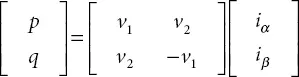
Where
p = Active power demand
q = Reactive power demand
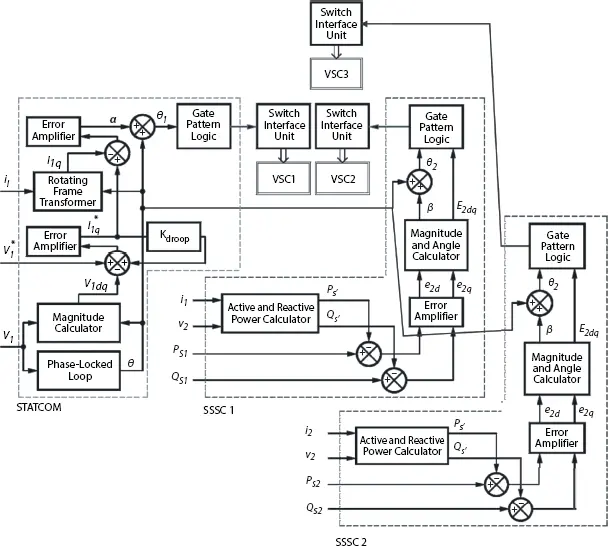
Figure 2.11 Basic control of GUPFC compensator logic.
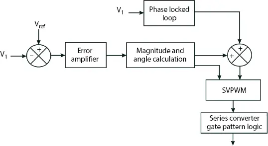
Figure 2.12 Basic control of series compensator logic.
v 1and v 2= Input voltage
i αand i β= Correction component.
The injected voltage angle can be calculated:
(2.16) 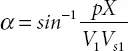
2.5.1.2 Shunt Converter
Figure 2.13indicates shunt converter pulse logic with basic control system. The reference voltage and current are compared with desired active and reactive power demand in the circuit. The shunt converter has ability to provide source or sink for system current.
Considering transformer admittance 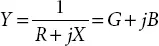 and bus volt age is V ∠ δ . The power injected using STATCOM can be shown to be [1]:
(2.17) 
(2.18) 
Where,
k = constant based on type of inverter (for six pulse converter  and Vdc ∠ α is veriable input voltage for transformer.
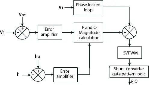
Figure 2.13 Basic control of shunt compensator logic.
2.5.2 Simulation of Active GUPFC With General Test System
The simulation study of active GUPFC system is carried out using MATLAB Simulink platform. MATLAB (matrix laboratory) is a multioptional numerical computing environment and programming language. It is developed by MathWorks Inc. MATLAB allows matrix manipulations, plotting of functions and data, implementation of algorithms, creation of user interfaces and interfacing with programs written in other languages, including C, C++, Java, Fortran and Python. An additional package, Simulink, adds graphical multi-domain simulation and Model-Based Design for dynamic and embedded systems. The simulations carried out with the following conditions and assumptions:
1 Hardware: Intel Core i5 2,450 M CPU, 2.5 GHz, 4 GB RAM with Win 7, 64 bit OS.
2 Software: MATLAB Simulink (7.10.0.499) 2010a release
3 Simulation time: 3.00 s
4 Simulation solver: ode23tb (stiff/TR-BDF2)
5 Simulation type: Variable step
6 Simulation relative tolerance: 1e−3: 0.001
The active GUPFC is simulated for the simplified general test system as shown in Figure 2.14. The test system parameters presented in the Appendix. With a grid connection, the system uses power for load feeders, whereas the system without grid connection continues to supply power to TPS auxiliaries using active GUPFC. Hence a load of TPS auxiliaries is always taken care of by active GUPFC.
The system illustrated above is simulated for two phases to a ground fault with phases A and B (R and Y) and phases B and C (Y and B) using MATLAB Simulink. The simulation conducted without GUPFC, with GUPFC and with active GUPFC for common test conditions. The combined result is plotted with load voltage against time and illustrated in Figure 2.15. The sequence of events is as shown in Table 2.2.
2.5.3 Simulation of Active GUPFC With IEEE 9 Bus Test System
With IEEE 9 bus test model, as shown in Figure 2.16, various fault conditions such as three-phase to ground fault and single-phase to ground fault are simulated with and without grid connection using MATLAB simulation, as illustrated in Figure 2.17. The results are presented for test cases with and without GUPFC, with and without fuel cell (distributed generation) and with active GUPFC. Three-phase to ground fault shown from 1.0 to 1.5 s on time axis whereas single phase to ground fault shown between
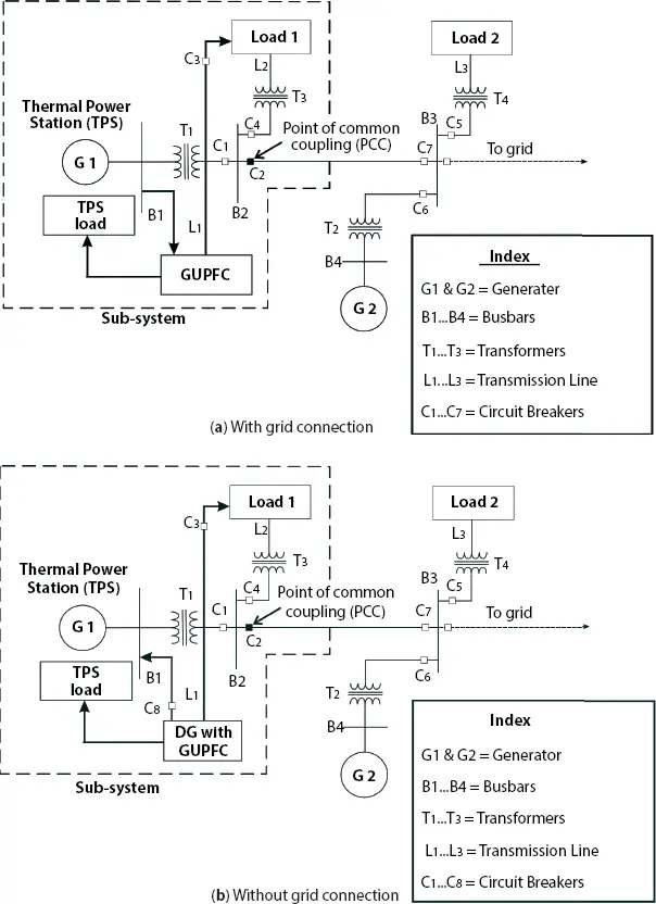
Figure 2.14 Simplified test system.
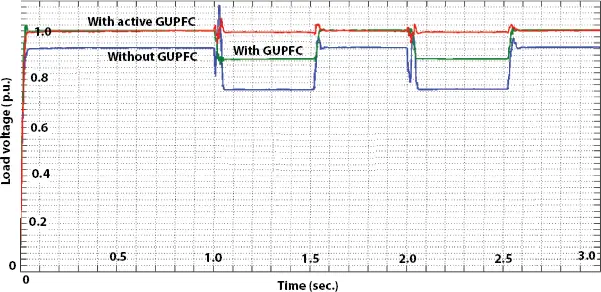
Figure 2.15 Test system simulation.
Table 2.2 Test system simulation events.
| S. No. | Time (s) | Event |
|---|---|---|
| 1 | 0.00 | Start |
| 2 | 1.00 | Fault on A and B phases |
| 3 | 1.02 | CB opens (disconnect sub-system from main system) |
| 4 | 1.50 | Fault Clear |
| 5 | 1.52 | CB close (connects sub-system to main system) |
| 6 | 2.00 | Fault on B and C phases |
| 7 | 2.02 | CB opens (disconnect sub-system from main system) |
| 8 | 2.50 | Fault Clear |
| 9 | 2.52 | CB close (connects sub-system to main system) |
| 10 | 3.00 | End |
2.5.3.1 Test Case: 1—Without GUPFC and Without Fuel Cell
Интервал:
Закладка:
Похожие книги на «Microgrid Technologies»
Представляем Вашему вниманию похожие книги на «Microgrid Technologies» списком для выбора. Мы отобрали схожую по названию и смыслу литературу в надежде предоставить читателям больше вариантов отыскать новые, интересные, ещё непрочитанные произведения.


Обсуждение, отзывы о книге «Microgrid Technologies» и просто собственные мнения читателей. Оставьте ваши комментарии, напишите, что Вы думаете о произведении, его смысле или главных героях. Укажите что конкретно понравилось, а что нет, и почему Вы так считаете.